How many of you had “Cuyahoga River catches fire” on your 2020 bingo card?
Yet that’s what happened today.
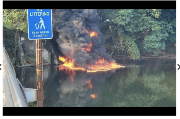
A tanker-car collision/fire near the Cuyahoga River in Akron this morning spilled burning fuel into a storm sewer and then the river, so the river caught fire. This is the first time in 51 years and 2 months that the Cuyahoga River has burned.
When it comes to fires on the Cuyahoga River, the burning river jokes are inevitable. But there are some real, substantive differences between this small fire and the fires of 50+ years ago.
Today we have a clear point source of the fuel and fire making it into the otherwise nonflammable river in Akron.
50+ years ago, there were many, many point sources & non-point sources of pollution that made the river itself flammable (in Cleveland, near the mouth), and all it took was a sufficient spark. The Cuyahoga burned more than once (13 times before today), and so did rivers in other industrial cities in the US.
The Cuyahoga’s historical fires made it the burning river that “sparked” the environmental movement in the late 1960s/early 1970s. Both local grassroots and national efforts have led to dramatic improvements in water quality since then. The Cuyahoga River still has some issues, but flammability isn’t among them. NE Ohio is justifiably proud of the rebirth of its rivers and its history of environmental work. And we should be.
Today’s event reminds us that we need to keep our environmental protections strong and not backslide on regulation. We need to fill the gaps in those regulations, not widen them.
River fires need to remain extraordinarily rare, small, easily-contained events that are sobering reminders of our history, not re-enactments.
And today’s events should spur us to better manage stormwater, so that the river to roadway connection is indirect, not a pipeline for a blaze. The same connection that allowed burning fuels to reach the river today, allows road salt, metals, and many other pollutants to enter the river every time it rains or the snow melts. These direct connections between roads and rivers are everywhere and they are a major remaining source of pollution for rivers like the Cuyahoga. If you care about the health of rivers and streams (and apparently, if you don’t want them to risk catching fire), you should be pushing for stronger stormwater management, including retrofitting stormwater controls into existing roadways and developed areas.
If you want to learn more about the environmental history of the Cuyahoga River, I highly recommend this documentary. Today’s accident and fire occurred a short distance upstream of the Akron Gorge Dam, which features in the film as one of the last major impediments to water quality on the middle river. The dam is currently slated to be removed sometime in the next 3 years or so.
[Photo by Cuyahoga Falls Fire Department, via Akron Beacon Journal. Story here: https://www.beaconjournal.com/…/one-dead-in-fiery-route-8-n…. My heart goes out to the families of the people killed and injured in the accident, and my sympathy goes to those who faced the disruption of evacuation from nearby homes and workplaces or a significant time spent stuck on the road.]
The location of this earthquake seems a little odd because North Carolina is about as far as it’s possible to get from an active plate boundary – thousands of km from the mid-Atlantic spreading ridge to the east and the San Andreas/Cascadia strike-slip subduction combo to the west.
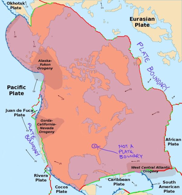
The extent and boundaries of the North American plate. Modified from original on Wikipedia.
The whole point – and power – of plate tectonics is that most geological activity, including earthquakes, occur at the boundaries of the Earth’s tectonic plates. Those plates are constantly moving and rearranging, but they are rigid enough to do without changing shape.
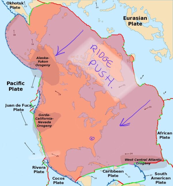
However, it is more accurate to say that they do so without changing shape much. “Intraplate” earthquakes like this one, or the M5.8 that shook Virginia in 2011, show that in reality, the interiors of plates can buckle and stretch. It just happens at much, much slower rates than at their boundaries. No matter where we are, the crust under our feet is always under stress. In the eastern US, the main source of horizontal stress is “ridge push” from the mid-Atlantic ridge, which has a roughly NE-SW direction.
Direction of ridge push force from mid-Atlantic ridge on the North American plate. Modified from original on Wikipedia.
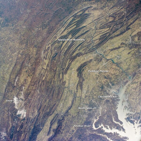
Normally, the interior of a plate is strong enough to take this stress, and transmit it onwards. But not always! The exceptions mostly occur in continental crust, which hangs around accumulating tectonic damage – faults & fractures – that make it weaker. Several times in the past billion years or so, this part of North America has been much closer to a plate boundary than it is now. Most obviously, the Appalachians are a testament to a continental collision about 350 million years ago.
Satellite view of the Appalachians, centred on Pennsylvania. Source: NASA Earth Observatory
But after the Appalachians formed, this region was stretched by the rifting that eventually formed the Atlantic Ocean; and the older rocks that the Appalachians is built from record earlier collisions & rifts. These past brushes with plate boundaries have left plenty of faults that could be reactivated by the forces currently stressing the tectonic plates.
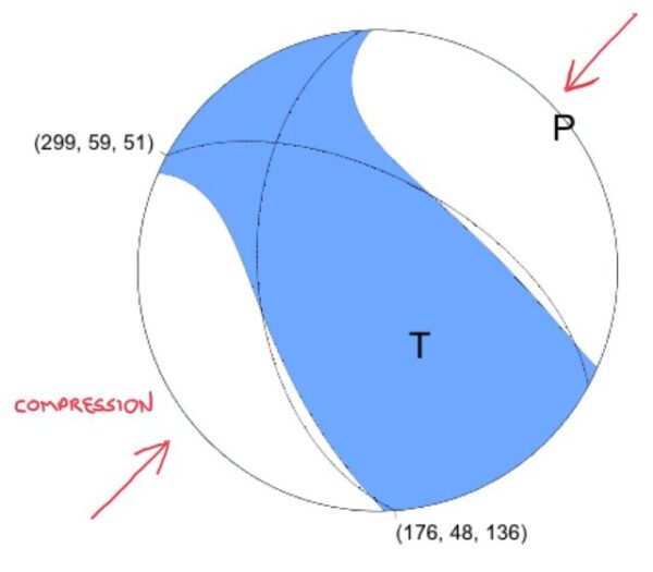
So we have stress, and structures that can potentially accommodate that stress. The focal mechanism indicates NE-SW compression on a reverse fault.
The direction of compression is consistent with the expected stress direction in this region due to ridge push. But as most of the old faults and structural boundaries in this region are also oriented NE-SW – the trend of the Appalachians – we might expect strike-slip faulting on a reactivated fault trending parallel to the stress direction, which seems to be a common type of earthquake in this region, rather than thrusting at right angles to the general regional trend.
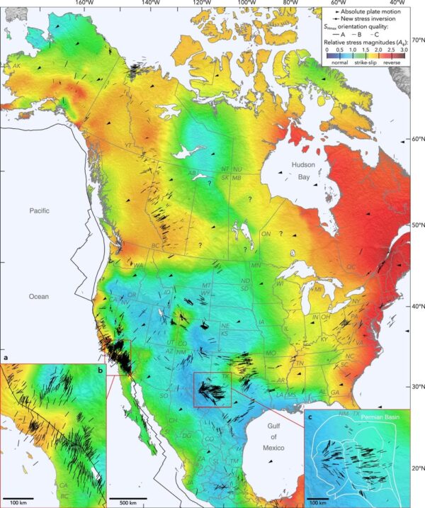
So yesterday’s earthquake was a bit of an outlier. One possibility comes from the fact that this is not a perfect double couple mechanism. It could be due to a problem with data coverage, or it could indicate that something more complex, involving multiple faults with different orientations, is going on. Zooming out, however, it seems that compressional intraplate faulting is actually quite common to the east of the Appalachians- see the red region in the figure below.
The basins created in this region by continental rifting as the Atlantic started to open in this region were linked together by NW-SE trending transform faults and lineaments (at least in Pennsylvania – I’m less familiar with subsurface structures in North Carolina). Perhaps one of these is being reactivated – at least to me, this seems more likely than entirely new faults forming.
Anyway, to sum up:
we expect earthquakes like this every so often.
this one is at least broadly reflecting the known regional stresses.
it is a little bit weird, but intraplate earthquakes tend to be an idiosyncratic bunch.
Establishing the rift valley and the mid-ocean ridge that went all the way around the world for 40,000 miles…You can’t find anything bigger than that, at least on this planet.
Lots of cool science history in this first-person account, but also some less cool stuff. Marie Tharp saw early on what the sea floor was telling us, but was dismissed with casual sexism?
Almost everyone in the United States thought continental drift was impossible. Bruce initially dismissed my interpretation of the profiles as “girl talk.”
Check.
Ideas taken much more seriously when a man starts to advocate for them?
We made profiles of some of the valleys in East Africa and noted the topographical similarities between the valleys in the ocean and on land. Bruce also noticed that the shallow earthquakes associated with the East African Rift fell within the valley walls. He began to endorse the existence of a continuous central valley within the mid-oceanic ridge.
Doc began to get interested at this point. He’d heard of this “gully,” as we called it, and he would pop into our lab from time to time and ask, “How’s the gully coming?”
Check.
Vulnerable people becong collateral damage in a feud between two male egos?
Now our efforts were thwarted by a long-lasting falling-out between Bruce and Doc. There are two sides to that story, but the result was that Doc banned Bruce from Lamont ships and denied Bruce access to Lamont data. He tried unsuccessfully to fire Bruce, who had a tenured faculty position at Columbia, but he did fire me.
Check out @IRIS_EPO's latest science highlight! Scientists discovered numerous previously unknown submarine landslides in the Gulf of Mexico that were triggered by earthquakes that were *super* far away! https://t.co/u62I5HFLVM
— Alka Tripathy-Lang, Ph.D. (@DrAlkaTrip) May 26, 2020
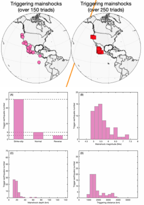
Earthquakes triggering landslides is not a surprise, but surface waves from a magnitude 5.5 earthquake in the Gulf of California triggering a landslide in the Gulf of Mexico (1500 km away) certainly is. This was but one of 65 earthquakes between 2008 and 2015 that were shown to trigger landslides (the landslides were identified and located from their seismic signature). The locations and characteristics of these earthquakes, from figures 4 and S6 of the paper, are shown below. I’m not sure if dominance of strike-slip is anything more than what you’d expect for tectonic situation in the source areas (not just the San Andreas and other inland strike-slip faults, but offshore fracture zones like the Mendecino)
Given that at the distances involved, the dynamic (temporary) stress changes from passing seismic waves will be very small, the local geology is a probably a big factor in amplifying their effects. In the Gulf of Mexico you have:
big piles of loose sediment, which will slow down & amplify passing seismic waves;
weak salt layers deeper down, which could act as easy failure surfaces for the overlying material;
and salt diapirs creating locally steep (and unstable) topography.
We have a region which is primed for submarine landslides. If only a small push is needed, perhaps distant seismic waves are enough to start things moving.
This study also shows the value of deploying (and maintaining) regional seismic networks: look at the cool stuff you find in all of that data!
One important thing to remember about this earthquake is that it happened in the era before we’d fully worked out plate tectonics. We were close, but there was still so much we didn’t quite understand.
Now we know that the deep trenches found off the coast of places like Chile are just the surface manifestations of giant thrust faults that dip very shallowly into the Earth – the subduction zones where the oceanic crust created at the mid-ocean ridges tens of millions of years before is returned to the mantle from whence it came. We didn’t know that then.
Now we know the recipe for giant earthquakes: you need fast plate motions and a long, shallowly dipping fault, which results in a huge surface area where the rocks stay shallow and cold enough to fracture, rather than flow, when stressed. Subduction zones are where these ingredients are present, so are where the Earth cooks almost all of the largest earthquakes. We didn’t know that then, either.
We also didn’t know that because the trenches are where these massive faults reach the seafloor, a large rupture pushes up a massive bulge of water that then rapidly collapses outwards – a tsunami. This amplifies and extends the deadly reach of the giant earthquakes. We – tragically – didn’t understand which earthquakes generate the large tsunami, and why.
This earthquake, and another large subduction earthquake in Alaska 4 years later, provided the key evidence for large horizontal motions on large thrust faults at subduction zones: a building block of what became plate tectonics. But these events also helped us to understand earthquake hazards much more clearly. We still can’t predict when big earthquakes will happen, but now we can understand where they happen, and what they do. This means we can save lives – through informed preparation before, warning of imminent tsunami during, and disaster response after. Today, an event like the Valdivia earthquake would be shocking, and devastating. But, at some level, we can at least comprehend that is it something the planet can do, in places like this.
We’ve come a long way since 1960.
The Earth’s long and drawn out response to a giant earthquake
Did you know that even after 60 years, the Earth is still ‘feeling’ the effects of this massive earthquake? Plate motions are slow and continuous, but the faults are not perfectly smooth. There is a stop-start cycle of slowly building up elastic strain that is suddenly released in abrupt, energetic earthquakes once enough strain has built up to overcome friction on the fault surface
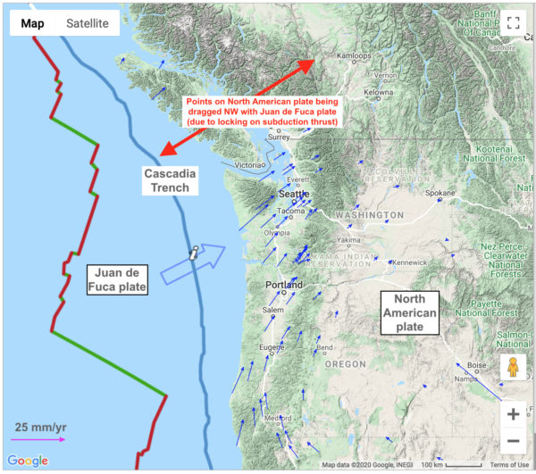
It’s been 320 years since the last big Cascadia quake, and GPS data shows it building up for the next one. The subduction thrust is locked by friction, so the coast on the overriding North American plate is being pushed inland as it moves with the subducting Juan de Fuca plate.
Map of the Pacific North west, showing northwest motion of GPS stations above the locked Cascadia subduction thrust. Source: UNAVCO
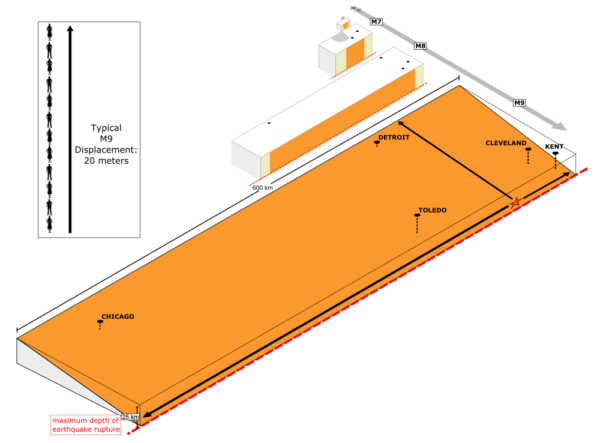
When a giant earthquake earthquake finally happens, the accumulated strain is released and the deformed part of the overriding plate rapidly heads back seawards, as we see here for the M9 Tohoku earthquake in 2011.
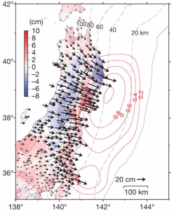
But here’s where it gets interesting: that seaward motion doesn’t stop when the earthquake does. Here’s GPS motions for the three months following the 2011 magnitude 9 Tohoku earthquake. The motions are much slower – centimetres in months rather than metres in minutes – but they are still in the same direction, suggesting they are a continuation of the process set in motion by the rupture.
Seaward (south-east) motion of GPS stations in Japan in the three months after the 2011 magnitude 9 Tohoku earthquake. Red colours show where there is uplift accompanying the horizontal motion; blue where there is subsidence. Source: Ozawa et al., 2011
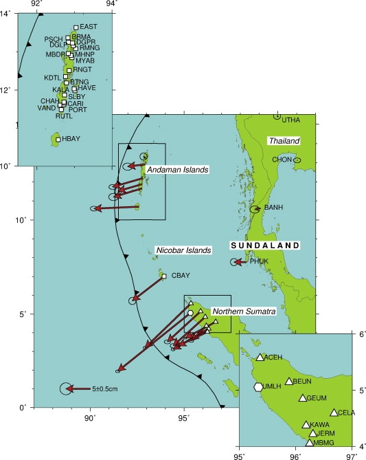
This is not an isolated observation: here’s data for a year after the 2004 magnitude 9.2 Sumatran earthquake which shows similar seaward motion.
Arrows show seaward (southwest) motion of GPS stations in Indonesia between early 2005 (just after the December 2004 M9.2 earthquake) and early 2006. Source: Gunawan et al. 2014.
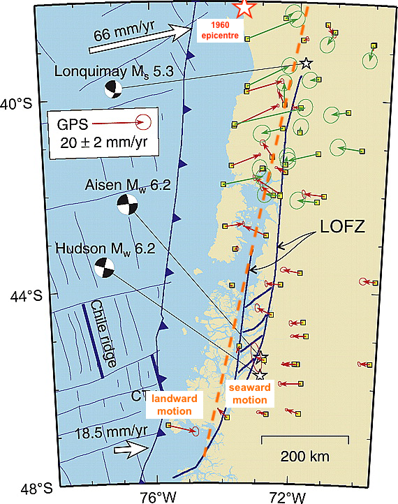
Some of this motion is due to afterslip: further motion on the fault surface itself. Many aftershocks are a response to this, but some weaker – or weakened – parts of the ruptured surface will creep aseismically as well. But the massive stresses imparted by these earthquakes also affect the deeper warmer parts of the Earth that flow – rather than fracture – in response to this change. Afterslip effects die away quickly with time, so after a few years this ‘visco-elastic’ response dominates. Furthermore, this flow can continue for a very long time from a human’s (or an earthquake’s!) perspective. Which is where the 1960 Chilean quake comes in. GPS data show that the inner coastal region is still moving seaward rather than landward.
Orange dotted line shows the transition from GPS stations currently moving landward (east, closer to coast) and stations moving seaward (west, further inland) in region ruptured in 1960 Valdivia earthquake (red star shows approximate epicentre). Source: Wang et al., 2007
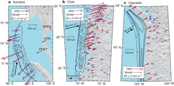
This figure from an excellent overview of the “Subduction Earthquake Cycle” allows GPS data from Cascadia, Sumatra, and Chile at different points in their earthquake cycle to be directly compared. The only thing to be careful about is that there are two sets of arrows on these figures: the red arrows show the actual observed motion, and the blue arrows show the results of modelling that includes a visco-elastic component due to flow of the mantle.
Sumatra one year after a giant subduction zone earthquake; Chile after forty years; Cascadia after 300 years. Source: Wang et al 2012.
