In Spring 2020, my Watershed Hydrology class transitioned to online in mid-March. This spurred me to create more blog posts and YouTube videos to provide content for the remaining units of the course. This substantial effort added to work I had been doing over the past several years to provide online resources to students in the class. Before we moved to fully online instruction, the goal of my blog posts were to free up class time for hands-on activities, by moving some of the methodological topics online. Obviously, after we moved online, the goal of my materials was to teach all of the content that I thought it was important for students in my class to know.
In this blog post, I provide links to the blog posts I had previously written for teaching purposes on precipitation, evapotranspiration and other topics and a listing of the blog posts I created during Spring 2020, including those with all of my resources on soil moisture and infiltration, streamflow generation, streamflow, and flooding.
How I taught Flooding online in Spring 2020 (this post has everything I did and includes links to the other blog posts under this heading, so if you want one-stop shopping, this is the link to click)
Note: The blog post above contains a number of links to other posts (not listed here) with many case studies of particular floods and flood generating mechanisms.
This post is part of a series in which I provide the details of each unit I taught post-transitioning to online in Spring 2020 in the Watershed Hydrology class at Kent State University. For more context about the course and my perspective on it, please read the introductory post. [I’ve added some bracketed notes about things I’d change up for a future online offering.]
[For 2020, this was the last section of my watershed hydrology course. (Sometimes, I have time for a specific unit on tracers and/or water quality). This is a little bit of a weird unit in that I included some content on analyses you can do with streamflow data before shifting to a focus on floods. This had more to do with evening out content vs. time than any innate splitting of streamflow analysis topics and/or grouping with floods. I do not expect students to do any of the analyses I talk about here, except some basic flood frequency analysis, but I want them to know the many ways that streamflow data are used and that they could explore in advanced class, in graduate research, or in their careers.]
In this unit, we explore:
more hydrological analyses you can do with streamflow data
basic flood definitions
flood frequency analysis (focus of associated problem set)
how we measure floods when there is no USGS gage (or it is wiped out by a flood)
what causes floods, and
how we manage floods
Learning Objectives
List several analyses that can be done with
streamflow discharge data, other than hydrographs and flow duration curves
Discuss how graphical- and tracer-based
hydrograph separations work and the insights gained from each
Identify some of the data inputs required for
watershed hydrological modeling, river forecasting, and hydraulic modeling
Describe the criteria used to distinguish
between National Weather Service flood levels
Demonstrate how to conduct a flood frequency
analysis and interpret the results of one
Identify why discussing floods in terms of
probability and not recurrence interval is considered the best practice
Give examples of situations that require caution
when calculating flood probabilities
Describe two methods that can be used to
estimate flood flows when there is no stream gage
Describe the common ways that meteorological
floods are generated and the spatial and time scales associated with each
Discuss
the role of topography and human land use in modulating flood dynamics
Identify
how climate change may be altering flood frequency and severity
Compare
flood control reservoirs, levees, and natural flood management as approaches
for managing floods
More hydrological analyses you can do with streamflow data
In this video, I talk about some of the ways that stream discharge data can be used to gain insight into processes occurring within a watershed. I talk about graphical and tracer based hydrograph separation, recession analysis, and hydrological modeling for what-if scenarios and river forecasting. You won’t know the details of how to do the analyses after watching the video, but you’ll know what sorts of possibilities exist.
Want to follow along with the slides? They are here (PDF), but I do recommend the video to get the context of the text and images on the slides.
More about river forecasting
The National Weather Service combines weather forecasts, watershed models, and stream gage data to make predictions of future flows at many locations around the US. This video takes you inside a river forecast center to learn more about how they operate.
What is the definition of a flood?
To kick off our course content on floods, start with this video. If you just want the slides, they are here (PDF).
How to do a basic flood frequency analysis
This was the need-to-know content for the last problem set for my students. If you just want the slides, they are here (PDF).
This is a blog post I wrote a while ago about flood frequency. It reinforces some of the things I talk about in my video lecture.
Some important cautionary notes about flood frequency analysis
Now that you know how to do a flood frequency analysis, you shouldn’t just blindly do one with any dataset you can find. Here I talk about some cautions.
In this short blog post, devastating flooding moving downstream in Pakistan’s Indus River watershed is an example of the timescales and effects of flood wave propagation. Flood wave propagation comes up in my cautionary notes video above.
The Red River of the North and its annual ice-jam floods comes up in my cautionary notes on flood frequency analysis video. Here’s a blog post I wrote if you want to read a little bit more about this interesting (and very flat) area.
How do we quantify floods when there is no streamgage?
At the end of my video on cautionary notes about flood frequency analysis, I mentioned some ways we can still estimate flood flows even when there’s no stream gage. The two videos below give you an overview of these important methods.
Hydraulic Models
This video discusses how hydraulic models are used for floodplain mapping and other engineering applications. Hydraulic models, which focus on the mechanics of flow within a channel(or floodplain!) are different than the hydrologic or watershed models I discussed in the “more streamflow analyses” video. Hydrologic models, that focus on the water balance in all parts of a watershed, can be used to provide the input data for a hydraulic model or even be coupled directly into the same computer program.
How to make an indirect measurement of a flood, using Manning’s Equation
In this video, a USGS hydrologist explains the basic theory and measurements needed to make an indirect measurement of flood discharge using the Manning’s equation. Please note that the constant of 1.486 only applies if you use English units. If you use metric units, the constant is 1. Because of course it is.
Note that there are a whole other set of flood generating mechanisms including dam breaks, glacial outbursts, landslide dams, and volcanoes that I don’t even cover here. You’ll just have to stalk my blog after the semester is over to see if I make good on my promise to write about them. Or ask me – I LOVE to talk about this sort of stuff.
Once you’ve read the blog post linked above, you may want to read more about some of the case studies I mention in it. I’ve linked many of them below for your combined reading ease. Note that these are all optional, but you may find them helpful to gain additional details on the concepts in the blog post above.
Optional reading if you want to know about one of the most spectacular floods ever. It will blow your mind.
How do we manage floods?
After all this talk of flooding, you might be asking, what can we do? This last section of the course is designed to help answer that and leave you with a realistic, but maybe hopeful, sense of how hydrologists, engineers, and environmental scientists can help manage floods by working with a watershed’s hydrology and landscape.
This video provides a good introductory overview of several approaches to flood management.
In this blog post, I use my hometown to discuss some of the risks of a heavy reliance on levees to manage flood risks.
How levees can make things worse
How do flood control dams and spillways work?
This video presents an engineering perspective on how flood control dams operate, how spillways work and how they are integral to the design and operation of dams.
One of the important things this video points out is the risk of dam or spillway failure. When such a failure seems like a real possibility, dam operators will do everything within their power to prevent the worst from happening, even if that guarantees that downstream flooding will get worse. This was part of the drama that happened in Houston during Hurricane Harvey.
[Note: I really wish I’d been able to accompany this content on the engineering of dams with some examples of how they change hydrographs in multiple different ways, but, frankly, I ran out of time to prepare that material and couldn’t find an already produced video or written piece that was appropriate. I’d love to know about one, if you’ve got one.]
Natural flood management: a (re)emerging trend
There are lots of opportunities for geologists and environmental professionals to become involved in natural flood management and many other exciting aspects of hydrology. Your training in watershed hydrology could be a launching point for a career managing water resources, protecting people, and improving the environment. But whatever you choose to do after this course is over, I hope that some appreciation for the way water moves through landscapes sticks with you. Thank you for being wonderful students this semester and know that I will be thinking of you for a long time after this semester is over.
Assessment
10 question multiple choice quiz, drawn from a bank of more than 10 questions. Students could take the quiz twice.
Problem set focused on flood frequency and qualitatively assessing uncertainties associated with estimating floods. This year, the problem set had the added bonus of a “record-breaking flood” on the stream we use in the problem set occuring after the end of 2019 water year. That allowed students to construct the flood frequency curve, then look up the 2020 flood discharge, calculate an estimated frequency for it, and then discuss how the assignment would change for next year’s class when that data point was included.
Questions on the final exam, including interpretation of a flood frequency graph.
Please respect my work
This work (my videos and blog posts) are licensed under an Attribution-NonCommercial-NoDerivs 3.0 Unported (CC BY-NC-ND 3.0). That means that you need to give appropriate credit if you use or modify anything I’ve posted here. It also means that you can’t use the material for commercial purposes. If you want to use other resources I’ve listed above, please respect the rights of the originators. If you want to use my sequencing of topics and resources in your class, by all means, go ahead.
This post is part of a series in which I provide the details of each unit I taught post-transitioning to online in Spring 2020 in the Watershed Hydrology class at Kent State University. For more context about the course and my perspective on it, please read the introductory post. [I’ve added some bracketed notes about things I’d change up for a future online offering.]
Finally, we’ve made it to the stream! This section of the course focuses on water flow in streams (streamflow, discharge, Q). We’ll focus on the following topics:
Why is measuring streamflow important?
Why does streamflow vary over time?
How do we measure streamflow?
How do we find streamflow data?
What are some hydrologic analyses we can do with streamflow data once we have it?
I have a fair number of different resources to cover these five topics, so I’m going to insert some sub-headers in the material below. You can use them to help you keep track of what you are supposed to be focused on.
Learning Objectives
List some of the ways that streamflow data are useful.
Explain why long term stream gauge records are important.
Describe what a water year is and why it starts when it does
Identify whether storms contribute a large fraction of total flow in urban streams
Explain how USGS stream gages work and how stage is measured
Describe why velocity varies in four dimensions and how velocity is measured
Explain the function of a rating curve or stage-discharge relationship
Demonstrate how to identify and download different types of data from the USGS NWIS website
Explain the appropriate uses, units, and graphical conventions for hydrographs, unit hydrographs, and hydro-hyetographs
Describe what a flow duration curve is, how to make one, and how to read the flow percentiles off of one
Why is measuring streamflow important?
Streamflow is of course an important output for watershed’s water balance. Plus, it’s a lot easier to measure that evapotranspiration, so accurate measurements of precipitation and streamflow, combined with some simplifying assumptions, can be used to estimate the actual evapotranspiration of an area.
It’s OK to geek out about streamflow data just because you have fallen in love with all things hydrology. But what are the practical reasons to measure streamflow? Why does the USGS operate over 8000 streamgages around the country? This webpage from the USGS Water Science School lists a bunch of really good reasons to measure streamflow and does a great job of slightly expanding on the topics of the video above.
This USGS Water Science School webpage gives a brief overview of why we need to measure streamflow every day for many years – because it varies seasonally and interannually (across years). In the associated problem set, I have students look at seasonal and internannual patterns of flow (but their graphs will look a little different than the ones the USGS made here, as I ask them to work in unit discharge in metric units.)
Why we need long-term streamflow data
I’ve teed this video up to a key excerpt about why we need long-term streamflow data. This is followed by some good comments about how climate change adds uncertainty to our understanding of streamflow regimes. (The rest of the video is great too, giving an expanded version of why streamgages are important)
In this USGS Water Science School webpage, you will learn about the magnitude of peak flow and total stormflow relative to baseflow. The page also talks about the characteristic flow regime of urban streams. Note that some streams, especially those sustained by a lot of groundwater, will have a very ratio of stormflow to baseflow over the course of the year.
How do we measure streamflow?
All the things you need to do to measure streamflow
I created this video during an online office hours session, which means that it is really long (50 minutes), has some hilariously bad attempts at drawing with a mouse and unfunny jokes, and there are slides (30 MB, PDF) to go with it. I advised students that it they didn’t want to watch the whole thing, they should look at the slides carefully and then identify the sections of the video they needed to watch in order to check their understanding or gain additional content.
After watching the above video (or not), you should take a look at the videos below that show actual USGS gages and streamflow measurements. You can also get the TL;DR version of how to measure streamflow on the page linked below.
What does a USGS gage look like and how does it measure stage?
I haven’t found the one perfect video that shows you everything I wished you could see about how a stream gage works, but here are two videos that let you peek inside a USGS gage. The first video gives you a good general overview:
This second video gives you the view from a USGS hydrologic technician as she checks on the gage and makes a streamflow measurement.
It is important to note that both of these videos show gages that operate with a stilling well. But USGS gages also use other technology (bubblers, ultrasonic) to measure depth. I just can’t find a video showing these.
Want to see what it actually looks like to make a streamflow measurement by wading or from a bridge? These two videos from the USGS give you a glimpse of the process.
How do we find streamflow data?
The following videos show how to find and access data from USGS stream gages via the National Water Information System. I designed these to be helpful for my students who are required to find, download, and manipulate USGS data in order to complete the associated problem set.
The USGS National Water Information System is the primary portal to streamgage data in the US. It’s important to understand the different ways you can identify a dataset to investigate – or just to see how much water is in your local stream or river.
In this video, I take you on a tour of the streamflow information you can find on the USGS NWIS website, using the Cuyahoga River at Jaite as our example gage. I talk you through what the graphs and tables on the current and historical observations page mean, how to see where the gage is located and look at the availability of other types of data, and then…very importantly for the problem set, I show you how to get to the daily data page, select the date range you want to examine, and save the data to your computer in a way that will be useful for opening in Excel or another spreadsheet program.
This video should help you get data into Excel or Google Sheets to complete the problem set 10. If you use a different browser or spreadsheet program, your may find that things are slightly different than what I do, but you can usually google or find a youtube explainer for how to do the file saving and importing.
If you use Google Sheets, create a new sheet, then go to file –> import data. Locate your saved txt file and then a menu like the one below should pop up. Leave everything as it is and click the big green “import data” button and you will have your data into columns properly. Then you can tidy it up as shown in the video above.
In this video, I show you three ways to examine the field measurements of discharge that underpin the continuous timeseries of streamflow you can find on the US Geological Survey (USGS) National Water Information Service (NWIS) website. I show you how to display the measurements on a graph of streamflow, where to see the actual rating curve, and the way to access the tabular data showing individual field measurements. Put together, all of these things should give you a small sense of how hard USGS hydrologic technicians work to produce good quality streamflow data.
What are some hydrological analyses we can do with streamflow data?
I have adapted these tutorials into my own guide (PDF) to making hydrographs, constructing flow duration curves, and conducting a flood frequency analysis. [Note: I discovered this year that some students got thrown off by the equation that told them to multiply the probability (P) by 100 to get to %. Then, when I told them that recurrence interval was 1 / P their numbers were incorrect. I will fix this in a future year.]
In the video below, I talk through some of the basic ways we can examine and analyze stream discharge data: hydrographs, unit hydrographs, flow duration curves, and runoff ratios. I provide some pointers on how to make effective and visually appealing graphs. This video shows the sorts of graphs students make as they work on the associated problem set.
10 question multiple choice quiz, with questions drawn from a larger bank. Students had the opportunity to take the quiz twice.
Problem Set in which students download daily USGS data from 2 streams, construct unit hydrographs and flow duration curves and compute some basic metrics. Students are then asked to write a few paragraphs contrasting the streamflow regimes and explaining why they see the patterns they do based on climate and landscape. Students have already delineated the watersheds and computed watershed characteristics using StreamStats in an earlier problem set.
Questions on the final exam.
Please respect my work
This work (my videos and blog posts) are licensed under an Attribution-NonCommercial-NoDerivs 3.0 Unported (CC BY-NC-ND 3.0). That means that you need to give appropriate credit if you use or modify anything I’ve posted here. It also means that you can’t use the material for commercial purposes. If you want to use other resources I’ve listed above, please respect the rights of the originators. If you want to use my sequencing of topics and resources in your class, by all means, go ahead.
This post is part of a series in which I provide the details of each unit I taught post-transitioning to online in Spring 2020 in the Watershed Hydrology class at Kent State University. For more context about the course and my perspective on it, please read the introductory post. [I’ve added some bracketed notes about things I’d change up for a future online offering.]
Overview of Streamflow Generation Unit
We’ve talked about how water goes down (precipitation), up (evapotranspiration), and down (infiltration). Streamflow is the last major term in the water budget – but before we can talk about streamflow we’ve actually got to get the water into the stream (or wetland or lake or …). That’s what we’re going to study now.
I made a video to introduce you to this topic and define a few key terms. Watch this first and then proceed to work your way down this page watching videos and reading content as you go.
Distinguish between baseflow and stormflow (also called quickflow) and explain when each occurs
Describe the conditions that generate infiltration-excess overland flow and where it is likely to occur
Describe how saturated overland flow works and explain how it is different than infiltration excess overland flow
Explain the requirements for subsurface stormflow and discuss the sequence of events that occurs for it to be produced
Discuss how the variable source area concept is related to subsurface stormflow and saturation overland flow
Illustrate the different connections that can occur between groundwater and streams and lakes
Explain how groundwater pumping can affect streams
Analyze how streamflow generation mechanisms affect stream peak flows and lag times
Define velocity and celerity in the context of hydrology
Discuss how climate, topography, soils, and geology influence the streamflow generation mechanisms that operate in a watershed
Examine how human actions can influence streamflow generation mechanisms and associated hydrograph characteristics
What is streamflow generation?
Terminology note: In the video above and in other resources listed below, you may see the phrase “runoff generation” used. I prefer the term “streamflow generation” because I’m interested in all of the ways that water gets to streams (or other water bodies), not just ways that involve surface runoff or overland flow. I also use the term streamflow generation to talk about how we get baseflow (i.e., water in the stream between storms), which is not runoff.
Required Reading
The Runoff Processes website (from the COMET international edition) has short pages of text accompanied by good animations of the processes being discussed. You should work your way through:
Overview of Runoff
Paths to Runoff
Basin Properties
Soil Properties (this should be a review from our infiltration section)
Modeling Concepts (recommended, but not required)
Summary
Take the practice multiple choice quizzes at the end of each section to check your comprehension.
You should also read Chapter 5 pages 125-138 in your Brooks et al. textbook, if you haven’t already done so.
More about Groundwater and How it Interacts with Streams
Every year, some students in my class have had a full hydrogeology course, while others know nothing about groundwater. I have struggled to find the right approach to teaching groundwater basics within the confines of a broader watershed hydrology class, while not boring/overwhelming my students depending on their background. I’ve decided that focusing on groundwater-surface water interactions is the way to go. The video below by Ken Bradbury provides an excellent introduction to the topic and I think hits the mark better and more concisely than I have ever done in person.
The video was produced by the American Geosciences Institute (AGI) and is actually part of one of three that together make a nice hour-long seminar on Water as One Resource, with multiple presenters. You can access all three parts, the associated slides, and even quizzes through the AGI Geoscience Online Learning Initiative website. Ideally, I’d love to have students complete the whole sequence, which I think would be appropriate for both those with and without a hydrogeology course under their belt. But in the interest of simplifying log-ins and content during this highly unusual semester, I opted for just the video shown above.
I’ve written this as a blog post to help you make the connection between what’s happening on/in the hillslopes to what happens in the stream. The different flow generation mechanisms affect the way a stream responds to rainfall. How quickly does the water start to rise? And how high do the peak flows get? (Estimated reading time: 10-15 minutes)
This is another blog post I wrote, in which I try to put the flow generation mechanisms in context of watershed characteristics. We’ve been talking about watershed characteristics all semester long, and here is yet another way that they are important for understanding (or even predicting) what happens in the streams. (Estimated reading time: 7-10 minutes)
Masterclass on Streamflow Generation
This is totally optional and not in any way required for anyone, but if you think that streamflow generation mechanisms are just about the coolest thing that you’ve ever heard of, then you can learn so much more about them from one of the world’s leading experts on hillslope hydrology: Jeff McDonnell in this 3 hour short course (requires flash).
When I was a graduate student I got to take a 10 week hillslope hydrology class with Dr. McDonnell and it changed the way I think about the world beneath my feet. Listening to 3 hr recorded presentation isn’t nearly as good, but you could still learn a lot if you want to do a deep dive.
Assessment
A 10 question multiple choice quiz, drawn from a bank of more than 10 questions, which students had the opportunity to take twice.
Questions on the final exam.
I don’t have a problem set that accompanies this unit, but I’d love to hear how others treat this topic quantitatively or in terms of data interpretation in a similar course.
Please respect my work
This work (my videos and blog posts) are licensed under an Attribution-NonCommercial-NoDerivs 3.0 Unported (CC BY-NC-ND 3.0). That means that you need to give appropriate credit if you use or modify anything I’ve posted here. It also means that you can’t use the material for commercial purposes. If you want to use other resources I’ve listed above, please respect the rights of the originators. If you want to use my sequencing of topics and resources in your class, by all means, go ahead.
This post is part of a series of posts in which I provide the details of each unit I taught post-transitioning to online in Spring 2020 in the Watershed Hydrology class at Kent State University. For more context about the course and my perspective on it, please read the introductory post. [I’ve added some bracketed notes about things I’d change up for a future online offering.]
Learning Objectives:
By the time you’ve worked your way through these materials, I expect you to know how to:
Explain the relationships between the concepts of gravity drainage, capillary water, adsorbed water, saturation, field capacity, and wilting point.
Give examples of how a sponge can be used to demonstrate infiltration and soil moisture concepts
Diagram a vertical profile from the land surface to the saturated zone, identifying important zones for hydrologic processes
Describe how volumetric water content, matric potential, and pressure potential change throughout the vertical profile.
Discuss how soil properties influence infiltration capacity.
Explain why hydraulic conductivity is affected by the water content of the soil
Recall the key difference between the Horton Equation and Green-Ampt equation
Summarize the key assumptions and features of the Green-Ampt equation
Explain why each of the variables in the Green-Ampt equation (for vertical infiltation with ponding) appears where it does in the equation.
Describe how a Guelph permeameter and double ring infiltrometer work
“Lecture Slides”
“Lecture Slides” for Soil Moisture and Infiltration(18 MB, PDF). [Note: These are the slides I was planning to use and had posted for my class before we went online. I keyed the resources I posted for my students to the slide numbers here, so student could cross-reference my slides and whatever video or blog post they were looking at. After this unit, I abandoned unit-long slide decks.]
Soil Moisture Concepts and Measurement (slide 2)
This 25 minute video was recorded in 2018, and was part of a several year effort to shift the time I was spending in class talking about measurement techniques out of the classroom. I wanted to make more time for fundamental concepts and hands-on explorations during our 75 minute class periods. In a normal year, I would go over the concepts in class, and then send them to the video for review of the concepts and info about the measurement techniques. I have a question on the problem set that asks the students a question about the measurement techniques that is very answerable if they’ve watched the video and paid attention.
Soil Water Potential (slides 4-6)
This 17 minute video introduces the concepts related to soil water potential and provides a worked example of a simple problem.
The link above is to a blog post I wrote that steps you through a diagram of the unsaturated zone and the relevant water content and water potential states of each part of the vertical profile.
There is also a short video, by Oregon State’s John Selker, that talks about the unsaturated zone more generally and it may be helpful if you are feeling a bit lost.
On our last day of in-person class, we broke out a bunch of sponges, water, and cafeteria trays for catching the mess and played with simulating the various moisture states of soils. We also watched how the wetting front propagates downward during infiltration and used some strangely water-repellent sponges to discuss hydrophobicity. The website linked above has photos and descriptions for those not able to take part in class, but I think this activity is one that could fairly easily be done by students at home (as long as they have a sponge) in an online course.
The link above is to a blog post I wrote on hydraulic conductivity. The blog post contains a nice video explanation by John Selker of why unsaturated hydraulic conductivitiy is lower than saturated hydraulic conductivity. The blog post also contains another video by John Selkerthat tells you more about the soil water characteristic curves shown in slide 15. [We talked a little bit about soil water characteristic curves, but they are an example of the sort of content that I expect graduate students to spend more time learning than the undergraduates in this course.]
Soil Bulk Density Increases and Hydraulic Conductivity Decreases with Depth (slide 26)
Up near the surface, soils tend to be “fluffy” – plant roots and animal burrows make lots of big pore spaces and there isn’t much pushing down to compact them. So near the surface, soils tend to be low density (1 g/cm3 is common – and that’s the density of water) and they tend to have relatively high hydraulic conductivity.
As you go deeper, plant roots and animal burrows go away and the overlying soil starts to squeeze and compact the pore spaces. As a result, soils get denser and have lower hydraulic conductivity. The soils are still a lot less dense than solid rock though – quartz has a density of 2.6 g/cm3. But once you get past 1.4 g/cm3 plant roots have a hard time getting through the soil .
Of course, what happens at the surface can really change the vertical profile. In the images in the slide, notice how the grazed soils have higher bulk density and lower hydraulic conductivity near the surface. Animal feet are good at squishing those fluffy surface soils.
Read through the five very short web pages (linked above) on how soil properties affect infiltration and runoff generation. You’ll learn about soil texture classification, soil composition, soil profiles, and surface properties. There are even some review questions you can use to check your understanding. [These web pages were produced by the COMET program, international edition. We also came back to this website when we discussed runoff generation in greater detail.]
Macropores are some of my favorite things. The link above takes you to a page built by Cornell’s Todd Walter. It does a really nice job of explaining what macropores are, why they are important, and it provides some pictures. If you want to know more about other types of preferential flow (finger flow, funnel flow), you can follow the links at the bottom of that page.
The video below was taken by one of my former graduate students, at his field site. I love to see classroom knowledge being applied in the real world. And the excitement!
Infiltration equations (slides 33-35)
This video by Oregon State’s John Selker talks about the Horton Infiltration equation (slides 33-34) and how it is empirical – which means that it based on measured data and relationships, without reference to any physics. Other infiltration equations (like the Brutsaert one in the video), the Richards Equation (slide 35), and the Green-Ampt equation (slides 36-44, Problem Set 8) are fundamentally rooted in physical understanding of how infiltration works. So the Horton equation can give you a good answer (if you have the data to put into it), but it can’t tell you *why* infiltration works the way it does. For that we need a physically based equation.
Introduction to Green-Ampt (slides 36-39)
This video by John Selker does a pretty good job of setting up the Green-Ampt equation and the assumptions that make it a physically reasonable, but not mathematically impossible representation of reality. Note that in the video, he focuses on the horizontal case (like near an irrigation furrow) which simplifies the math a little bit relative to the case of vertical infiltration (like for rainfall), that is shown in your slides. [I wish that there was a similarly excellent video for the vertical case, which is more relevant to the natural phenomena of infiltration.]
More Green-Ampt (slides 40-41)
This video by John Selker goes into a bit deeper detail mathematically about how the Green-Ampt equation works. Again, he uses the horizontal case, which simplifies things further than I do on the slides. But he does show some of the math involved in getting the equation into a useful form.
[I encouraged graduate students to work their way through the video and the derivation linked below, but made the material optional for undergraduates this semester. I didn’t feel confident that students could watch and read the material without much chance at interaction – in a different form than in the slides and textbook – and not come away with some confusion and/or apprehension. If I were to teach this unit online again, I would make sure to align my content with Selker’s videos and/or make my own.]
The link above takes you to Todd Walter’s course notes on the Green-Ampt equation. This is a pretty thorough, yet well organized and digestible treatment of the math. As noted above, I made this material optional for undergraduates this year.
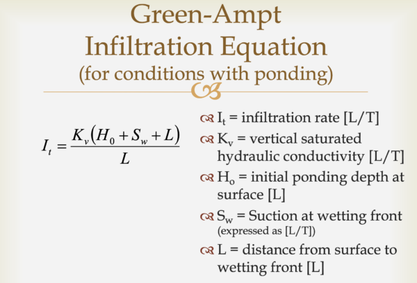
The main Green-Ampt Equation to know (slide 42-44)
Concerned I might be overwhelming students with Green-Ampt derivations, I wanted to draw their attention back to a fairly simple form presented in my course slides. Make sure you’ve followed the slides and videos enough to know where K and L come from and why Sw and Ho are in the equation.
The above link takes you to a blog post where I explain how double ring infiltrometers and Guelph permeameters work, and remind you about the definitions of infiltration capacity and equilibrium infiltration capacity. I also have some nifty videos of them in action, including one of my students from a previous year.
Assessments
Students’ understanding of the material in this unit was assessed in three ways:
a problem set with four parts: (1) presenting soil moisture data time series and asking for interpretation of it; (2) using an Excel spreadsheet (that I provide) with the Green-Ampt equation embedded to change soil properties and assess the effects on infiltration; (3) using the same Excel spreadsheet to conduct a sensitivity analyses on the effects of initial water content and rainfall rate and explain their results; and (4) sending them to the Web Soil Survey and a target area of interest to assess what information relevant to the Green-Ampt equation they can find readily versus what requires assumptions of appropriate values (e.g., from a textbook table) or specialized measurements.
a 10 question multiple choice quiz that I wrote to align with the learning objectives. There were more than 10 questions in the test bank and students could take the quiz 2 times.
questions on a midterm exam that spanned evapotranspiration and this unit.
Special thanks to…
Many of the amazing videos for this unit were made by Dr. John Selker of Oregon State University. You can learn even more about soil hydrology and biophysics from him at https://www.youtube.com/channel/UCoMb5YOZuaGtn8pZyQMSLuQ/playlists. And thanks also to Dr. Todd Walters of Cornell University for his clear images and explanations linked above. You’ll see more from him in the next unit on streamflow generation mechanisms.
Please respect my work
This work (my videos and blog posts) are licensed under an Attribution-NonCommercial-NoDerivs 3.0 Unported (CC BY-NC-ND 3.0). That means that you need to give appropriate credit if you use or modify anything I’ve posted here. It also means that you can’t use the material for commercial purposes. If you want to use other resources I’ve listed above, please respect the rights of the originators. If you want to use my sequencing of topics and resources in your class, by all means, go ahead.