9 isotopes fractionating

A post by Chris RowanOn the 9th day of Christmas my true love sent to me: 9 isotopes fractionating…

Many elements exist in the form of two or more isotopes. Different isotopes have the same number of protons and electrons, so chemically will react in the same way, but their nuclei contain different numbers of neutrons, giving them different atomic masses. For example, the simplest and most abundant element in the Universe, hydrogen, has three isotopes with zero, one and two neutrons in their nuclei, giving the isotopes atomic masses of one (protium), two (deuterium), and three (tritium), respectively.

500px-Hydrogen_Deuterium_Tritium_Nuclei_Schematic.svg.png
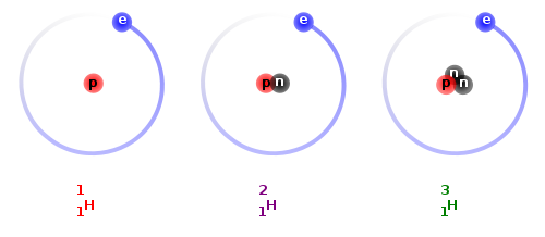
Hydrogen, Deuterium, Tritium. Source: Wikipedia

The different atomic weights of isotopes allows mass spectrometers to separate them from each other (their ions are deflected slightly different amounts by an applied magnetic field) and measure their relative proportions in a sample. And, as it turns out, the ability to measure isotopic ratios is a rather useful tool, and not just for dating zircons. Just as in a mass spectrometer, physical processes can fractionate many isotopes, so that they are distributed in different proportions in different reservoirs (physically or chemically distinct parts of the Earth’s biogeochemical systems), such as the ocean and the biosphere, the crust and the mantle, or even the Earth and the rest of the solar system. This enables the influence and contribution of different reservoirs to be measured, and new ones to be identified. Changes in the distribution of isotopes between different reservoirs over time can be used to track the rates of different geological processes that have produced the fractionation. Here is just a flavour of the sort of things you can investigate using the isotopic ratios of different elements, some of which have been discussed on this blog before.

  • Carbon. Life, or more specifically, the enzymes that drive cell biochemistry, generally prefer to use lighter isotopes at the expense of heavier ones. Because of this, organic matter is enriched in 12C relative to 13C. Isotopically light carbon is thought to be a distinctive product of biological activity, and such material found in 3.85 billion year old rocks in western Greenland, is possibly evidence for very early life: the only evidence that could possibly be found, given how much the rocks they are found in have been altered by heat and pressure.

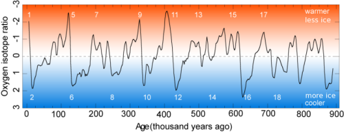
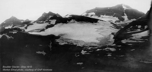
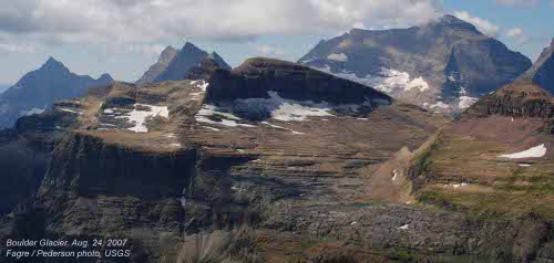
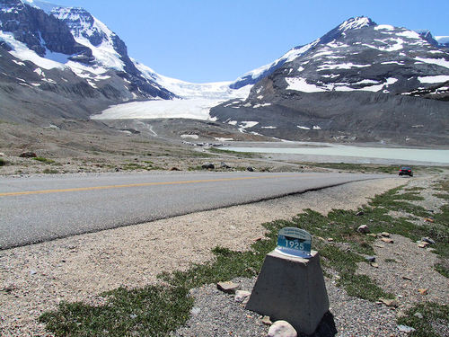
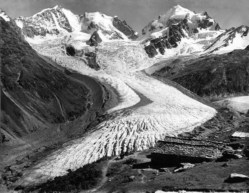
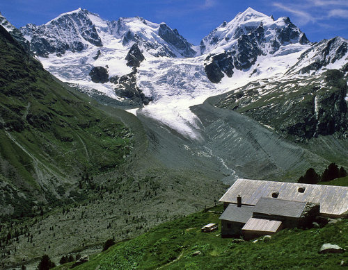
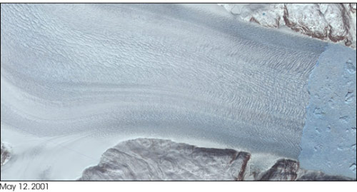
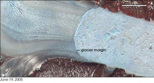
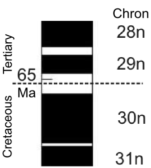
  • Oxygen. Water cycle processes that involve change of state between solid, liquid, and gas fractionate oxygen isotopes. Evaporation from the ocean favours lighter isotopes, so when the Earth’s ice caps grow, they form from snow that is enriched in 16O relative to 18O. This in turn enriches the ocean water that is left behind. The ratio of 18O to 16O in the oceans therefore increases and decreases as the polar ice caps wax and wane, and these variations are recorded by carbonate in the shells of marine organisms such as foraminifera, allowing climatic fluctuations to be measured and dated.
  • oxygen_isotopes.png
    Source: INGV

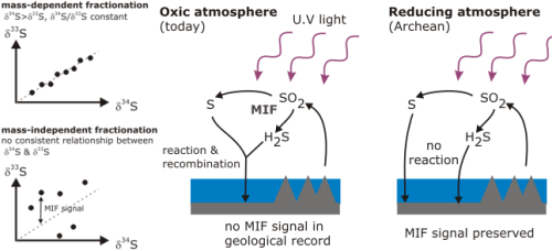
  • Sulphur. Purely physical processes in the upper atmosphere cause mass independent fractionation of 32S, 33S, and 34S, in contrast to reactions involving sulphur at the Earth’s surface. In today’s oxygenated atmosphere, all the compounds fractionated in the upper atmosphere quickly recombine with each other, but when the Earth’s atmosphere was anoxic, they remained separate. Mass independent fractionation of sulphur isotopes is observed in most sediments older than about 2.5 billion years, and the disappearance of this signal in younger rocks provides a highly sensitive marker of when oxygen first began to accumulate in the Earth’s atmosphere.
  • MIFcomb.png

  • Osmium. On a planetary scale, isotopic studies take advantage of the fact that the Earth is differentiated, meaning that when the planet formed a lot of heavy elements ended up in virtually inaccessible reservoirs such as the core and lower mantle, with most of the surface stocks of these elements being produced by radioactive decay of other elements since the Earth’s formation. Thus reservoirs on the Earth’s surface have markedly different isotopic ratios than the deep Earth, or undifferentiated extra-terrestrial material like chondritic meteorites. Following this principle, excursions in the ratio of 187Os to 188Os of seawater can be used to detect asteroid impacts, and even estimate the size of the impactor. Most of the osmium on the Earth’s surface is 187 Os which has been produced by radioactive decay of rhenium since the planet’s formation; an asteroid contains much more primordial 188Os. Thus an impact leads to large negative excursions in the marine 187Os/188Os record.
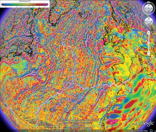
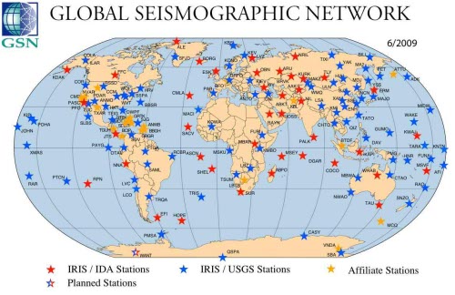
impactOs.jpg
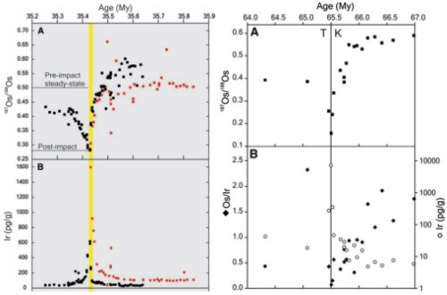
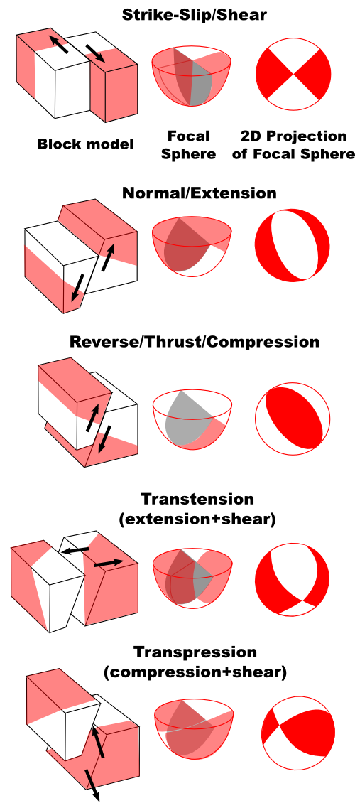
Source: Francois et al., 2008

Isotope geochemistry is an extremely versatile and powerful tool – once you’re armed with a mass spectrometer, you can use it to attack a wide variety of geological problems, and many diverse processes, although in terms of my abiding interest – tectonics – they are perhaps less informative than my palaeomagic, even though I suspect that a rock’s magnetism is reset much more easily than its isotopic ratios…

8 streams reversing,

7 glaciers melting,

6 fields a-flipping,

5 focal mechanisms,

4 index fossils,

3 Helmholtz coils,

2 concordant zircons,

and an APWP.

Categories: geochemistry, geology, planets

8 streams reversing

A post by Chris RowanOn the 8th day of Christmas my true love sent to me: 8 streams reversing…

Wind gaps are fossil rivers: water once flowed through these valleys, but now that water has been diverted to flow elsewhere.

Wheeler_wind_gap.jpg
Wind Gap in Wheeler Ridge, California. Source (HT to my co-blogger Anne)

Each of the triangles on the drainage map of northern California (from a 2006 paper by Lock et al.) below marks a wind gap that occurs mid-way along a continuous north-south trending channel.

F4.large_.jpg
Figure 4 of Lock et al. (2006)

On either side of these dry sections, water in the channels to the north flow north, and water in the channels to the south flow south. But this doesn’t always seem to have been the case: the deposits left by these stream systems contain signs of their flow directions in the past, paleocurrent indicators that show that a few million years ago, water in the currently south flowing sections also flowed north, as did water in the wind gaps before they were dry. At some point, the streams south of these wind gaps have reversed themselves.

Ridge1.png

In their paper discussing the origin of these features, Lock et al. argue that their formation was the result of a relatively recent uplift event altering the drainage patterns of pre-existing streams and rivers. Initially, the high ground was in the south, and water drained northwest all the way from here into the sea. But over the last few million years, something has caused the ground in the middle of the area to rise up as the ground in the south subsided. This created a wind gap-bearing barrier to water flowing from further south, and by reversing the topographic slope in this area, forced the streams there to turn back on themselves, so that they now flowed south.

Ridge2.png

So, what caused this uplift? Northern California is actually parked right on top of a rather interesting tectonic situation: it marks the spot where the boundaries of three tectonic plates intersect with each other. To the north is a subduction boundary, where the Juan de Fuca plate is being thrust beneath the Cascades. To the south, the Pacific and North American plate are sliding past each other along the San Andreas Fault. Trending west out to sea from Cape Mendecino (CM in the northwest of the drainage map above), the Gorda and Pacific plates move past each other along a ridge transform fault (the Mendecino fracture zone). Due to the presence of this triple junction, Northern California marks the boundary between two distinctive styles of deformation on the coast of west North America: subduction thrusting to the north, and strike slip motion to the south.

California-tectonics.jpg

The net result of the relative motions between the North American, Pacific, and Juan de Fuca plates is that the triple junction does not stay in the same place: in the last few million years, it has gradually moved northwards along the North Californian coast, lengthening the San Andreas Fault at the expense of the Cascade Trench. This migration squashes the crust ahead of it, causing uplift, and stretches the crust behind it, causing subsidence, causing a region of transient uplift to also gradually move up through northern California, reversing streams as it goes.
By tracking the changes in drainage by mapping, correlating and dating the river deposits in northern California, you can chart the passage of the triple junction with much higher resolution than is possible with other geological indicators. And given the interests of myself and my co-blogger, a study revealing an interesting and informative link between tectonics and hydrology is sort of perfect for this blog , don’t you think? Although if the hydrology stuff makes sense, it’s really only thanks to Anne’s editorial assistance – and if it doesn’t, it’s only thanks to me.
Lock, J., Kelsey, H., Furlong, K., & Woolace, A. (2006). Late Neogene and Quaternary landscape evolution of the northern California Coast Ranges: Evidence for Mendocino triple junction tectonics Geological Society of America Bulletin, 118 (9) DOI: 10.1130/B25885.1

7 glaciers melting,

6 fields a-flipping,

5 focal mechanisms,

4 index fossils,

3 Helmholtz coils,

2 concordant zircons,

and an APWP.

Categories: geology, geomorphology, paper reviews, tectonics

7 glaciers melting

A post by Chris RowanOn the 7th day of Christmas my true love sent to me: 7 Glaciers melting…

All over the world, where there are glaciers, those glaciers are not as large as they once were a century, or even a few decades, ago:

Boulder Glacier, Glacier National Park, USA

Boulder1910.jpg
1910

Boulder2007.jpg
2007
Source: USGS Repeat Photography Project

Athabasca Glacier, Canadian Rockies

Athabasca.jpg
Photo by Idle Moor, downloaded from Panoramio.

Tschierva glacier, Swiss Alps

tschierva_1880.jpg
1880

tschierva_2004.jpg
2004
Source: swisseduc.ch

(other retreating Alpine glaciers)

Helheim Glacier, Greenland

Helheim2001.jpg

Helheim2005.jpg
Source: NASA Earth Observatory

Upsala Glacier, Patagonia

Upsala.jpg
Source: JAXA Earth Observation Research Center

Gangotri Glacier, Himalayas

Gangotri.jpg
Source: NASA Earth Observatory

Tasman Glacier, Southern Alps, New Zealand

Tasman.jpg
Source: NASA

Glaciers are dynamic systems, but although there are some complexities in interpreting the behaviour of any individual one, when you see the same rapid shrinking trend in all of these different parts of the world, you stop looking for local causes.
As it is the New Year, and with the failure to reach any concrete agreement to cut our greenhouse gas emissions in Copenhagen still smarting, we should perhaps use this time to consider our own culpability in the mess. For until our leaders believe that they will gain more votes for making the hard choices than they will lose for damaging economic growth – until, in other words, we in the developed world start thinking that rather than becoming a little materially richer next year, it would be better if we made our planet a little less worse – the stalemate will continue. And whilst we rail against the failure of those we elect to curb our excesses, we buy more things, and use more energy, and worry if our economy does not grow at more than 3% a year. Somehow, no matter how much we have, there never seems to be a time when we will say, ‘we have enough’.
Perhaps the fault, dear readers, lies not within our politicians, but within ourselves.

6 fields a-flipping,

5 focal mechanisms,

4 index fossils,

3 Helmholtz coils,

2 concordant zircons,

and an APWP.

Categories: climate science, environment

6 fields a-flipping

A post by Chris RowanOn the 6th day of Christmas my true love sent to me: 6 fields a-flipping

About every millon years or so, on average, the Earth’s magnetic field reverses itself: the north magnetic pole becomes the south magnetic pole, and vice versa. The most visible evidence for this can be found in the world’s ocean basins, where the striped magnetic anomalies that provided compelling evidence for sea-floor spreading and mid-ocean ridges also provide a continuous history of the last 200 million years of so of geomagnetic field behaviour.

NAntMagAnomalies.jpg
Magnetic anomalies in the North Atlantic. Source: SDSU (link to kml file)

As I have explained before, ‘on average’ has no real predictive power: the field can spend only a few hundred thousand years in one polarity state before switching to the other, then right afterwards spend a few million years in that state before flipping again. At least as far as we can tell, there is no periodicity to field reversals. This very unpredictability does have a rather useful consequence, however. Because, at least as far as we know, there is no real periodicity to the field, over any particular period the temporal pattern of magnetic field reversals – how often the field reverses, and when – is unique to that period, and unlike the pattern in any other period. So if, for example, I am trying to date a sedimentary sequence that spans six magnetic polarity reversals, with mostly normal (shaded black) periods, or chrons, interspersed with shorter reversed (white) chrons:

KTmagstrata.png

from the temporal pattern of reversals – at least a medium normal, very short reversed, longish normal, medium reversed, medium normal, short reversed, at least a long normal – I can fairly confidently match it to the series of reversals that occurs over the KT boundary. As long as your sequence spans enough polarity chrons, that pattern is not going to be like any over period covered by the geomagnetic polarity timescale (GPTS) principally constructed from measurement and dating of the seafloor magnetic anomalies.

KTmagstratb.png

This is effectively what magnetostratigraphy is all about: locating polarity reversals within a sequence and matching the pattern of polarity reversals to the existing. Reversals are extremely good chronological markers: they are usually well-dated, occur virtually instantaneously from a geological perspective (a few thousand years is not very significant if you’re looking at a sequence spanning a few million) and, most importantly, mark a global event that is simultaneously recorded by rocks forming in all sorts of ways and environments. Magnetostratigraphy is therefore especially good for long distance correlations between sequences that record environments so different from each other that the same index fossils may not be present in them.
The sequence of seafloor magnetic anomalies is often described as a magnetic barcode, and in a very real sense it can act as one: with the right palaeomagnetic tools, you can read the age of a geological section directly from the recorded sequence of reversals.

…5 focal mechanisms,

4 index fossils,

3 Helmholtz coils,

2 concordant zircons,

and an APWP.

Categories: geology, palaeomagic

5 focal mechanisms

A post by Chris RowanOn the 5th day of Christmas my true love sent to me: 5 focal mechanisms…

The global network of sesimometers pick up on any largish earthquake and allow people like the USGS to triangulate their location and work out their magnitude.

GSN_6-2009_map.jpg
Source: IRIS

Data from these stations can also be used to derive useful information about the nature of the fault that ruptured, usually provided in the form of beach-ball like focal mechanisms, which are based on the first motions of the seismic waves generated by an earthquake, which will be different at different seismic stations depending on their azimuth from the rupture point. For example, in the first block model of a strike slip fault in the figure below, the fault trends to the northwest and has ruptured with a dextral sense (from the perspective of someone standing on one side of the fault, the other side has moved to the right). Due to this rupture, rock in the northwest and southeast quadrant is initially compressed, before snapping back elastically, meaning that seismic waves transmitted in these directions have a squashy, compressional first motion. In contrast, rock in the northeast and southwest quadrants are initially stretched before elastically recovering, meaning that seismic waves transmitted in these directions have stretchy, dilational first motions.

With a good global distribution of seismograph stations, waves in all 4 of the compressional and dilational quadrants will be picked up, allowing the distribution of first motions, and hence the fault configuration, to be reconstructed. The focal mechanisms that are usually given to convey this configuration are a way of plotting the three dimensional fault information in two dimensions (they’re lower hemisphere stereographic projections). The figure below is an attempt to show how a simple block model of the first motions of 5 common types of earthquake look when projected onto a lower hemisphere, and then when the pattern on that focal sphere is projected onto the horizontal to produce a 2D focal mechanism.

5 common earthquake focal mechanisms

Why are focal mechanisms interesting? Because they allowyou to remotely determine the most common kinds of earthquakes occurring in particularly active areas, and hence how these areas are deforming in response to plate motions. This information is often not easily available in any other way: even if you visit an area, identifying active faults, and their sense of motion, can be a real challenge, and many fault ruptures might not even break the surface. Plus, they allow me to write posts like this.

4 index fossils,

3 Helmholtz coils,

2 concordant zircons,

and an APWP.

Categories: basics, earthquakes, geology, geophysics