5 focal mechanisms

A post by Chris RowanOn the 5th day of Christmas my true love sent to me: 5 focal mechanisms…

The global network of sesimometers pick up on any largish earthquake and allow people like the USGS to triangulate their location and work out their magnitude.
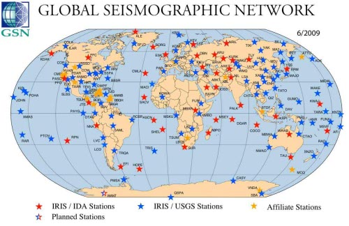
GSN_6-2009_map.jpg
Source: IRIS

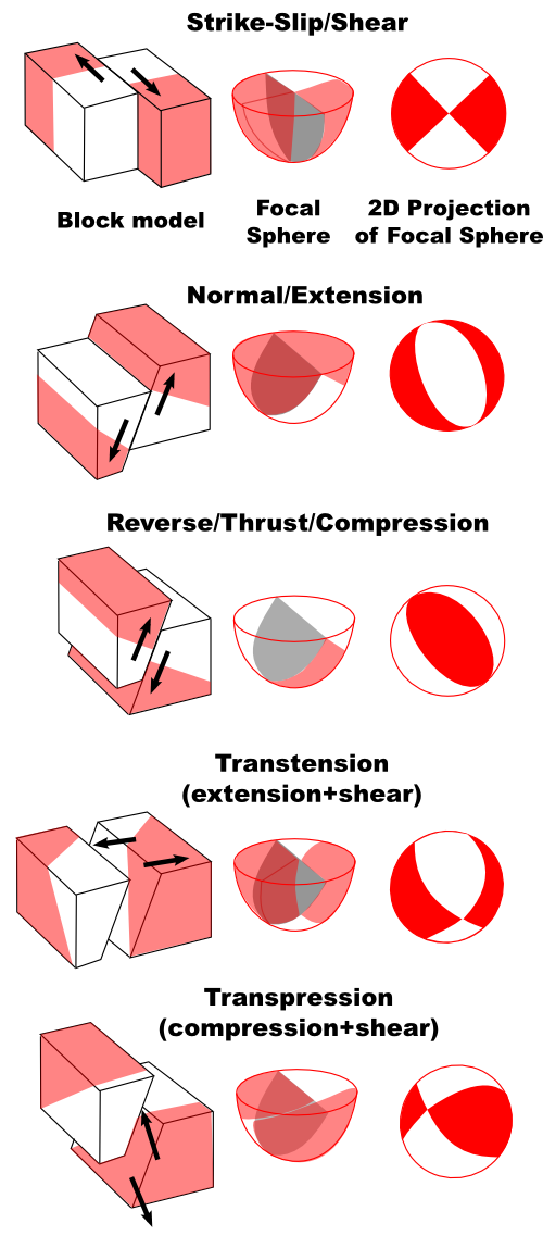
Data from these stations can also be used to derive useful information about the nature of the fault that ruptured, usually provided in the form of beach-ball like focal mechanisms, which are based on the first motions of the seismic waves generated by an earthquake, which will be different at different seismic stations depending on their azimuth from the rupture point. For example, in the first block model of a strike slip fault in the figure below, the fault trends to the northwest and has ruptured with a dextral sense (from the perspective of someone standing on one side of the fault, the other side has moved to the right). Due to this rupture, rock in the northwest and southeast quadrant is initially compressed, before snapping back elastically, meaning that seismic waves transmitted in these directions have a squashy, compressional first motion. In contrast, rock in the northeast and southwest quadrants are initially stretched before elastically recovering, meaning that seismic waves transmitted in these directions have stretchy, dilational first motions.

With a good global distribution of seismograph stations, waves in all 4 of the compressional and dilational quadrants will be picked up, allowing the distribution of first motions, and hence the fault configuration, to be reconstructed. The focal mechanisms that are usually given to convey this configuration are a way of plotting the three dimensional fault information in two dimensions (they’re lower hemisphere stereographic projections). The figure below is an attempt to show how a simple block model of the first motions of 5 common types of earthquake look when projected onto a lower hemisphere, and then when the pattern on that focal sphere is projected onto the horizontal to produce a 2D focal mechanism.

5 common earthquake focal mechanisms

Why are focal mechanisms interesting? Because they allowyou to remotely determine the most common kinds of earthquakes occurring in particularly active areas, and hence how these areas are deforming in response to plate motions. This information is often not easily available in any other way: even if you visit an area, identifying active faults, and their sense of motion, can be a real challenge, and many fault ruptures might not even break the surface. Plus, they allow me to write posts like this.

4 index fossils,

3 Helmholtz coils,

2 concordant zircons,

and an APWP.

Categories: basics, earthquakes, geology, geophysics

4 index fossils

A post by Chris RowanOn the 4th day of Christmas my true love sent to me: 4 index fossils…

Sometimes when you are studying a geological sequence, the most basic problem you need to address is establishing a reliable chronology – not just how old it is, but how much geological time is spanned not only by the whole sequence, but by specific beds or horizons within it. Only then can you start to examine the possible rates of environmental changes, and correlate them to changes in other sequences in the same region, or around the world. A good chronology needs as many well-dated ‘tie-points’ as possible; dating volcanic material is all well and good, but if your section contains one datable volcanic ash at the top, and all the interesting stuff is happening at the bottom, it’s not particularly helpful.
This is where biostratigraphy comes into its own. Particularly in marine sequences, fossils are much more abundant than datable horizons, and there exist several groups of organisms that provide highly useful and precise time stamps for the rocks they are found within, because they combine a wide geographic range (allowing regional or even global correlations) with fast rates of evolution, such that within quite a short time (geologically – it’s still usually at least a million years or two) some easily distinguishable physical characteristic changes markedly enough that they are classified as another species. These index fossils are therefore wonderful tools for filling in the chronological gaps.
Different index fossils are useful for different periods of earth’s history. One of the more common groups used when studying sediment cores brought up from the seabed (which range in age from 180 million years to essentially modern), are foraminefera, single-celled plankton with hard calcareous shells, and a very large diversity of morphological forms

forams.jpg
Source

Going further back in geological time, one of everyone’s favourite fossils, the Ammonoids, are extremely useful index fossils for Late Paleozoic and Mesozoic sequences, such as southern England’s Jurassic Coast. Many different species are easily identified by the different, and often highly intricate. patterns of their sutures – the lines where the walls of the chambers in their shells connect to the outer shell.

ammonite_suture.jpg
Source 1, 2

For the early Palaeozoic, graptolites – free-floating colonial organisms that populated the world’s oceans in the Ordovician and Silurian periods, between about 490 and 370 million years ago – are firm favourites.

Graptolite.JPG
Source 1, 2

Even generally fossil poor Precambrian rocks may contain potential index fossils, in the form of Acritarchs. This is not a ‘natural’ fossil group, in that everything that is identified as an acritarch is not necessarily closely related in evolutionary terms; a good working definition of them would be ‘organically walled microfossil that we’ve found but can’t really identify, and the ‘Acritarch’ actually means ‘of uncertain origin’. Palaeontologists’ best guess is that they’re probably mainly algal cysts. However, even if this group does contain lots of different ancient single-celled organisms lumped under the same banner, their fossil record stretches back into the Precambrian (the oldest known lived more than 2 billion years ago), possibly allowing for some biostratigraphic correlation between sequences from a time otherwise distinctly lacking in a fossil record, including the Neoproterozoic where I’m currently working.

acritarch1.jpg
Source 1, 2

3 Helmholtz coils,

2 concordant zircons,

and an APWP.

indextime.png
Useful time ranges for index fossils mentioned in this entry

Categories: fossils, geology

3 Helmholtz coils

A post by Chris RowanOn the 3rd day of Christmas my true love sent to me: 3 Helmholtz coils…

If you’re trying to measure the often rather weak magnetisation of rock sample, the last thing you need is other magnetic fields invading your measurement space and mucking up your readings. To avoid this, the magnetometer is placed in a magnetically shielded space. One method of doing this is to build a shielded room with walls made out of a material with high magnetic permeability, such as Mu-metal or transformer steel, that absorbs most of the magnetic flux before it encroaches inside. However, cost or space issues sometimes make this impractical.
An alternative is to generate your own magnetic field around the magnetometer, such that it cancels out the ambient field in your lab. For this to be effective, you need to have a set-up that will generate a uniform cancellation field within a volume large enough to fit your measuring equipment, which means that you employ paired Helmoltz coils. With the right separation, if you run a current around the coils a uniform axial magnetic field is created in the region between the coils.

Helmholtz.jpg
image source

In order to cancel out the ambient magnetic field completely, therefore, you need three pairs of Helmholtz coils, nested within and oriented perpendicular to each other. If you’re feeling fancy, you can even set up an active control system that will automatically account for changes in the ambient field: both natural changes due magnetic fields of the sun and moon, and the solar wind, interacting with Earth’s magnetosphere, and unnatural ones due to lorries parking outside your lab, cars moving past, or those crazy physicists down the hall.

Helmholtz cage.JPG
image source

With such a control system in place, most of the time you can reduce the magnetic field inside the coils from around 50,000 nano-tesla to less than 50 nano-tesla, which is just as good as being inside a mu-metal box. However, it is a slightly less stable low field environment, because rapid fluctuations in the field will sometimes occur too fast to be corrected for. My last two laboratories had magnetometers in shielded rooms, whilst my current laboratory in Edinburgh has a set of Helmholtz coils; so over the next few months I’ll be able to check their relative effectiveness for myself.

2 concordant zircons,

and an APWP.

Categories: geology, geophysics, palaeomagic

2 concordant zircons

A post by Chris RowanOn the 2nd day of Christmas my true love sent to me: 2 concordant zircons…

If you want to accurately date a rock, you really want to grind it up and extract some grains of zircon. This mineral has several useful properties: it is very hard and chemically inert, even at quite high temperatures, so will survive relatively intact even if the rest of the rock it is surrounded by is extremely squeezed, squashed and metamorphosed.

Zircons.JPG

image source 1, 2

In addition, zircon’s crystal structure allows lots of uranium to be trapped within a grain when it forms, but virtually no lead. This doesn’t mean that you don’t find any lead within zircons if you chemically analyse them – you do. But this lead was produced within the crystal after it formed, by the radioactive decay of uranium. In fact, two different decay processes are at work: uranium 238 decays to lead 206, uranium 235 decays to lead 207. Therefore you have two ways of getting a radiometric age for the zircon: you can measure the ratio of uranium 238 to lead 206, or you can measure the ratio of uranium 235 to lead 207. This means that zircons have a built in cross-check: if you calculate the age using both of these ratios, and they are the same within error, the age is said to be concordant, and you can have more confidence that the age you have determined reflects the original age of formation (a resetting event would affect the different ratios to a different degree, and result in discordant ages).
We’re currently trying to extract some zircons – or baddeleyites, which are similarly useful for dating but more common in mafic rocks than zircons sometimes are – from the dykes I sampled in Oman last year. Of course, I could probably do with more than two, but two would be a start!

and an APWP.

Categories: geology, rocks & minerals

An APWP

A post by Chris RowanOn the 1st day of Christmas my true love sent to me: an APWP

APWP stands for ‘apparent polar wander path’. The remanent magnetisation imprinted on a rock as it forms points towards the magnetic pole, and from its direction you can calculate where, geographically, the pole that the rock ‘saw’ falls on the Earth’s surface. Often, the pole position you calculate from the magnetisation directions of older rocks is some distance from the current geographic poles. It would have plotted there just after the rock formed, but after millions of years of plate motion, the continent it formed on is now at a different longitude and latitude, and hence a different distance from the geographic poles, than it was long ago. This phenomenon is called ‘apparent polar wander’, because it looks like the magnetic pole has moved with respect to the Earth’s surface, although in fact it is the Earth’s surface moving relative to the Earth’s magnetic pole.

pole2.png
A remanent magnetic pole which originally plots at the geographic pole will plot away from it after millions of years of plate motion

By plotting the magnetic poles for a sequence of rocks formed over tens or hundreds of million years, you get a record of continental motion over geological time: an apparent polar wander path or APWP. And if you can obtain APWPs for two different continents spanning a similar age range, you can get an idea of differential motions between them. For example, the APWPs for Europe and North America have a very similar shape between about 350 million and 100 million years ago (the sections of the lines furthest from the current geographic pole in the figure below), when they were both part of the supercontinent Pangaea and henced moved as one; indeed, if you close up the Atlantic Ocean that now separates them, the two paths will overlap.

Nam-Eur-APWP.jpg
Apparent Polar Wander Paths for North America and Europe since the Permian.

The project I’m working on at the moment is currently trying to generate APWPs for the different continents in an earlier time period, between 1000 and 500 million years ago. So this palaeomagician would love an APWP as a Christmas gift – although any sensible true love would certainly point out that I’m the one being paid to produce such a thing…
Note: this series is intended to be a light-hearted , and mildly educational, list of useful geological things. Hopefully, you don’t get too bored of this bit of seasonal whimsy before 12th night – if indeed you bother to check your RSS feeds before then!

Categories: geology, palaeomagic