When Kent State “pivoted to online” in mid-March, I was about half-way through my Watershed Hydrology class. For context, this class typically has about 20-25 undergraduate students, from geology, environmental studies, and conservation biology majors, and about 5-8 graduate students from geology and geography. I use the first part of the Brooks et al “Hydrology and the Management of Watersheds” textbook, which students have access to as an e-book through the Kent State library, but I don’t rely heavily on assuming the students are reading it. My goal for the 2020 edition of my class was to feature a hands-on activity in the classroom approximately weekly. That unfortunately, went out the window when we pivoted online in mid-March.
Side note: I really appreciated that Kent State and other universities distinguished between our suddenly online classes (which we called “remote instruction”) and classes that were intentionally designed to be delivered 100% online. But for simplicity’s sake, I’m just going to call it online on the blog.
What I did
When we went online, I decided to use an asynchronous approach so that
students could work through the material at times that worked best for them,
and then use class time for “online office hours” where students
could optionally come and get help with concepts and problem sets. I used a mix
of videos I created and those by others, blog posts I wrote and existing web
pages to support their learning. I wrote out learning objectives for each unit
(~1 week of material) and created a multiple choice quiz that they could take 2
times to check their understanding of the material. Each week the students also
had to a problem set tied to the concepts of the unit, but I made those
deadlines soft, recognizing that it would be easy for students to get
overwhelmed with everything going on during this turbulent semester.
We start the semester talking about the topographic definition of watersheds
and water and energy balances. Then we spend the rest of the semester working
our way through the water cycle, starting with precipitation and
evapotranspiration. So by mid-March, we were in the midst of discussing soil
moisture and just moving into infiltration. Because of the disruption
associated with moving online, I essentially just started the unit over when
classes resumed. Following that material, I had fully online units on
streamflow generation, streamflow, and floods.
Watch for upcoming blog posts to provide the resources and materials I used for each of the units that I taught on line.
Looking back
Am I happy with how the online portion of Watershed Hydrology played out in Spring 2020? More or less. I think given all of the constraints surrounding the rapid transition and circumstances of the online period meant that both I and my students did the best we could. I provided content, support, and grace for students to achieve what they wanted to achieve in my class this spring. To me, that’s the most important outcome.
Would I do the exact same thing if I had to teach Watershed Hydrology online again? No. I hope never to find myself in a position to pivot to online so suddenly again, without childcare, in the middle of a pandemic, so this was clearly not a thoughtful, best-case scenarios for teaching Watershed online. I am generally happy with the content I provided, though I might scaffold it differently in a future offering, as well as add/drop some things. I would certainly write a different syllabus in terms of expectations for a fully online class.
The biggest thing I would change is that I would add a larger synchronous component to the online course, particularly if the entire semester would be online. I did have an optional synchronous component to my 2020 class, that I billed online office hours, but held during the previously scheduled class period. During that time I was available via Blackboard Collaborate Ultra and able to answer questions about problem sets and other course content. Several students regularly attended those online office hours and found them very valuable, but other students never participated and only experienced the course asynchronously after the transition online. I was very sensitive to limitations in high speed internet access, increased family care and work responsibilities, and illness, and I want to acknowledge that those limitations will continue to exist. But I would like to find a way to have broader (if not complete) participation in synchronous sessions in any future online offering. I can envision using the synchronous sessions as an opportunity not just for students to get homework help, but also for students to work collaboratively on virtual “hands-on activities” involving data exploration (e.g., via Shiny apps) or internet-hosted modeling interfaces) or have group discussions based on videos that students had watched ahead of time.
While spring 2020 was incredibly rough on us as faculty and on our students, we can make future online hydrology experiences better for everyone by collaborative developing the needed tools and sharing our knowledge and resources.
Legendary fluvial geomorphologist Reds Wolman once said “Floods come from too much water,” and that’s the phenomenon distilled to its core essence. But this bit of wisdom doesn’t give us much to go on if we want to understand what creates floods or why some areas are more flood-prone than others. It’s the cooking equivalent to “Bread comes from flour.” How do we turn the flour into bread? How do we turn too much water into a flood?
In this blog post, I’ll create a cookbook for riverine floods, explaining the different phenomenon that generate floods and linking to examples that I or others have written about. I’ll be drawing heavily from the framework of a 2002 book chapter by O’Connor, Grant, and Costa called “The Geology and Geography of Floods” and as such I won’t be focused on the particulars of flood hydraulics or routing as the meteorologic, hydrologic, and geologic factors that are preconditions for floods. In a sense then, I guess I’m writing ingredients lists, not the full cookbook.
The first and most obvious ingredient you need for a flood is water. A lot of water. But if you have a lot of water draining slowly over time, that’s not a flood. It’s a river. So we need to have a lot of water, stored somewhere, and then release it quickly. Since the ways water can be released quickly are closely tied to where the water is stored, let’s start with storage.
Water can be stored as vapor in the atmosphere, liquid at the earth surface (in some sort of reservoir), or solid at the earth surface (i.e., ice or snow). That gives us a universe of three main types of floods: meteorological floods, dam break floods, and snow or ice melt floods. But those types are not absolute and bounded. You can have cross-overs. It can rain so hard as to burst a dam or rain on top of snow, melting the snow. But some floods are caused simply by too much rain, and these meteorological floods are the most common. That’s what I’ll cover in this blog post. (Look for volume 2 of the cookbook to cover how terrestrial water storage can lead to floods at some point after the semester is over.)
Meteorologial floods
Meteorological floods are closely tied to the four mechanisms of atmospheric lifting (convection, frontal systems, convergence, and orographic) that produce cooling, saturation, and precipitation. As climate change warms the atmosphere, enabling it to hold more water, and shifts atmospheric circulation patterns, there is the potential for more severe flooding and flooding in new places to result from any of these lifting mechanisms.
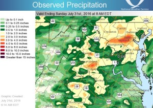
Convective rainfall + steep topography +/- human land use change = localized flash flooding
Precipitation that generated the 2016 Ellicott City flood. Ellicott City is in the reddest area, just to the west of Baltimore. (Image from the NWS.)
Clearly, convective storms can produce floods, and Ellicott City has terrible luck. But is it all bad luck? While the rainfall amounts from these storms are really big, if they’d happened in flat, sandy, forested areas, the resulting floods would have been much smaller. Unfortunately, historic downtown Ellicott City sits at the bottom on a locally steep valley that gathers runoff from three little tributary streams. And upstream, there is a lot of urban development. Ellicott City’s floods illustrate that the topography matters – the faster water runs down slope and gets collected into channels, the worse the flood will be, because more water will be entering the stream at once. Land use also matters, but for really extreme events, its signal is a little harder to parse, because if it rains hard enough or long enough, few landscapes will be able to infiltrate all of the water. Land use matters more for small floods.
Some convective storms are much larger than normal, and we call these “mesoscale convective systems” or “mesoscale convective complexes.” Mesoscale systems can have diameters of 10s to 100s of kilometers, and they can be major flood generators with impacts over much larger area than the isolated convective storms. The worst floods occur when large-scale atmospheric circulation patterns cause a mesoscale convective systems to stall out over a particular area, with thunderstorms popping up over and over again for hours or days. Isolated convective storms generally only cause floods for small streams, but an important feature of floods caused by mesoscale convective systems is that they affect more than one localized area, so they can create floods on larger river systems within or downstream of the area where rainfall occur.
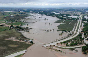
A stalled out mesoscale convective system over Colorado’s Front Range in September 2013 caused over 450 mm of rainfall in one week, resulting in over $2 billion dollars in flood damage and hundreds of landslides. Flooding started in mountain canyons where over 300 mm of rain fell in one 24 hour period alone. As all of that water drained onto the flat-lying plains, flooding continued for days in the South Platte River and its tributaries. Flooding occurred because of infiltration-excess and saturation-excess overland flow. Rainfall probabilities for this event are estimated to be >1/1000 years (though that’s extrapolating well beyond the data), but flooding probabilities are not quite that extreme, with most of the places where gages exist or estimates made having floods with a 1/50 to 1/500 year probability.
Damage from the 2013 Colorado floods in Boulder County, Colorado. (FEMA photo via Wikipedia)
Flooding near Greeley, Colorado from the South Platte River, September 19, 2013 (EPA photo via Flickr)
As with isolated convective systems, mesoscale systems can create bigger floods where topography is steep and there are lots of channels to quickly move precipitation falling on land into a stream network, resulting in more water arriving in the same part of a river at the same time.
Tropical and extra-tropical cyclones = flooding for miles and days
Tropical cyclone is the general term for hurricanes (wind speeds >74 mph), tropical storms (wind speeds 39-73 mph), and tropical depressions (wind speeds
Tropical cyclones are notorious flood generators, and inland flooding is the leading cause of death from these storms in the US. Hurricane categories only consider wind speed, not rainfall, so people may under-estimate the hazard associated with lower category storms. Immense rainfall totals can result as moisture is supplied to the storm by nearby ocean waters or by flooded and saturated soils on land. This makes slow moving hurricanes particularly dangerous flood generators, and it’s a reason that people are very concerned with the possibility that climate change could be contributing to slower hurricane movement after landfall. The most sobering example of slow-moving hurricane flooding in the recent past is Hurricane Harvey and its impacts on Houston in 2017. I wrote about the climate change connection and the land use connection at the time. Many fingers were pointed as Houston’s urban sprawl for worsening the disaster, and in some ways that’s fair (houses in floodplains are bad), but in other ways it’s not (almost nowhere can receive 1270 mm of rainfall in a few days without experiencing saturation and flooding).
Rainfall from Hurricane Harvey in the Houston area. By David M. Roth; NOAA WPC – http://www.wpc.ncep.noaa.gov/tropical/rain/harvey2017.html, Public Domain.
When tropical cyclones produce flooding in flat areas, like coastal plains along the East Coast and Gulf of Mexico, the floods can last for weeks. We’ve seen this repeatedly in the US, including prominently in North Carolina in 2016, following Hurricane Matthew.
Where tropical cyclones meet steep topography, spectacular flood destruction can result, such as when Hurricane Irene hit Vermont in 2011. Even though Irene dumped less rain on Vermont than where it first made landfall in North Carolina, the flood effects were much worse. A similar phenomenon happened just a week later in the Susquehanna River watershed, as a result of Tropical Storm Lee. In fact, those two storms prompted my first “recipe” for flooding: Take a tropical cyclone and add steep topography.
Atmospheric rivers + orographic lifting = a major source of floods for California and the Pacific Northwest
Atmospheric rivers are narrow bands of concentrated moisture coming off the ocean and onto land. They are an area of active research as we increasingly recognize how important they are for generating floods and building snowpacks in the Western US. Here’s a great explainer video:
A key thing about atmospheric rivers as flood generators is not just how much water they carry, it’s what happens as they are orographically lifted over steep terrain like the Coast Range, Cascades, and Sierra Nevadas. That lifting and cooling causes the moisture to come out of the sky and fall as rain and snow. If conditions are cold enough to form snow, skiers rejoice and hydrologists and emergency managers let out a sigh of relief. But often, the atmospheric rivers are coming from the tropical ocean, in what we call a “pineapple express”, so the moisture is not just abundant, it’s warm. Then, the precipitation falls as rain, even at high elevations, and we get floods. If an atmospheric river happens after snow accumulates in the mountains, it will melt some or all of the snow and we get even bigger floods.
Californians care a lot about atmospheric rivers, because they depend on mountain snowpacks and reservoirs to provide water for farms and people living in lower, warmer, and drier locations. But too much of a good thing is a flood. And climate change is projected to increase the intensity of atmospheric rivers affecting California and could even set up a scenario called the ARkstorm (for 1/1000 probability, atmospheric river storm). Watch the video below, because the consequences of this possible event are too big just to put into words, and yet, what could happen is based on state-of-the-art science and historical records of the 1861-1862 flood that inundated nearly the entire Central Valley.
Monsoon rains bring an average of 900 mm of rain to India each year. Spread out over the months of June to September, the rains are an important water source for crops, livestock, and humans, and helps offset the opposite season, when hardly any rain falls.
But when monsoon rains come in intense downpours, flooding can result. Some years, more rain falls or a lot of rain falls in the space of a few weeks, rather than more evenly spread out over months. In ways that we don’t completely understand, climate change seems to be making the monsoon rainfall less moderate and more sporadic. Dry periods interspersed with extreme precipitation periods are becoming more likely and that means that floods are becoming a more frequent part of the monsoon climate.
Monsoon flooding along the Chao Phraya River in Thailand, with July 2011 (left) and October 2011 (right) compared. Images are from NASA, via Wikipedia.
Important notes and take away points
These aren’t the only ways to cook up floods. First, I’ve only covered meteorological floods on rivers in this post, and then, I haven’t even covered all of those. Frontal systems can produce floods too, particularly if the ground is wet to begin with or if infiltration capacity is low. And rain-on-snow is a significant flood generator (even without the concentrated fire power of an atmospheric river) because the heat from the rain can melt large amounts of snow, dramatically increasing the volume of water contributing to a flood.
Climate oscillations like the El Niño-Southern Oscillation and Pacific Decadal Oscillation will exacerbate these flood generation recipes in some years and some regions, and mute them in other places. The climate oscillations don’t create flooding in-and-of themselves, but they can make things better or worse.
The recipes above will generate floods that vary in space and time scale of impact – from affecting headwater streams for a few hours to affecting huge river basins for months. In general, the highest intensities of rainfall will only affect a fairly small area for a fairly short amount of time, but mechanisms that produce more prolonged rainfall can cause widespread flooding, even if the intensity is lower.
Topography matters. Steep slopes route water quickly into streams producing high peak flows, while flat areas drain slowly resulting in floods that last much longer.
Land use matters – to some extent. In really extreme rainfall, it may make little difference in the peak flow and total flood volume, because the landscape would have been overwhelmed regardless of landcover. For smaller floods, land use, including deforestation and urbanization, definitely matters, and land use also matters quite a bit for things like landslides which often accompany floods. Regardless of size, a flood is a disaster when people are in the way, and land use is one rough proxy for how many lives and how much property is likely to be affected.
Climate change is affecting the frequency and/or severity of floods across all of these recipes, even if we can’t always detect the signal of climate change in a particular event. In general, we are seeing – and expect to continue to see – increases in extreme rainfall, the key ingredient in all of these recipes. And extreme rainfall intensity is increasing much faster than the overall increase in atmospheric moisture and mean precipitation. We are also seeing shifts in timing and location of flood-generating storms.
What drives the occurrence of slow-slip events on subduction zones: “earthquakes”: that involve strain release over days and weeks rather than seconds? A new paper…doesn’t really answer that question, but it shows why it’s so complicated to answer.
The study uses seismic and drill core data to characterise what is entering the subduction zone off the coast of New Zealand, where multiple slow-slip events that involve the shallow part of the subduction thrust have been observed. The idea is that what is about to be fed in to the trench will be similar to what is now just subducted. By sampling what’s on the seafloor, we get some insights into what the rocks currently controlling the behaviour of the subduction thrust are like.
On a broad scale, there’s a lot of variability to what is being fed in. The incoming plate has a lot of basement topography – it’s an oceanic plateau with lots of volcanic seamounts of various sizes and heights, with volcaniclastic sediments in betweeen. Carbonate-rich deep sea sediments deposited after the plateau formed have buried some but not all of the volcanic topography.
The drill cores confirm this broader spatial variability: the sequences within the two cores reported, about 15 km apart, varies dramatically, mainly because one samples a seamount and one does not. But within each core, there is also a lot of much smaller-scale variation in the volcanic and carbonate sediments. Big changes in alteration, and therefore important properties like porosity and seismic velocity, vary significantly within a few cm up or down the core.
What all this means: the geometry of the subduction thrust, and the properties of the rocks involved in faulting, change a lot in quite small area. It’s the geological equivalent of ‘garbage in, garbage out’: feed a subduction zone a complex plate surface, and you get a complex fault zone with complex behaviour.
Did the Earth have a magnetic field before 3.5 billion years ago? Previous paleomagnetic studies of the world’s oldest mineral grains – the Jack Hills zircons, which have maximum ages of 4.4 billion years – claimed that tiny inclusions of magnetite within those grains had taken a snapshot of a strong geomagnetic field at the time they formed.
Now, however, a new exhaustive study shows that we still don’t know, because the detected magnetisation came much later. The study shows that the carriers of the putative super-ancient magnetisation are not primary inclusions (crystallised from the melt first before the zircon grew around them), but magnetite formed by alteration later on. How much later? We don’t know. But it could have been any point between 4 billion years ago and today.
And thus, the state of the magnetic field in the Hadean and Eoarchean goes back to a big question mark. This is disappointing, but not totally unexpected. The fact that most magnetic minerals contain iron, and iron is redox sensitive, is a real bane for studying ancient magnetisations, because there is always the very real prospect that your rock is one age and the magnetisation you are oh-so-carefully measuring is another, younger, age. If you don’t realise this, then you are putting a continent or crustal block in the wrong place, or mischaracterising the magnetic field for the period you’re interested in. I have a certain amount of experience in this particular area.
This is a really nice example of how there is a distinction between ‘good’ data and meaningful data. Sometimes, you can have a really nice, precise measurement that nonetheless leads you completely wrong, because you lack the information to put it in the proper context.
Below I go through a list of important climate and landscape factors that influence flow generation, but I’m following in well-trodden footsteps in doing so. Dunne and Leopold (1978) created a classic diagram that puts it all together in a really elegant way. I encourage you to refer back to it as you read through the rest of this post and think about how each factor interacts with the rest to produce the streamflow regime that characterizes a watershed.
Runoff processes in relation to their major controls. Modified from Figure 9-16 in Dunne and Leopold (1978), by somebody I am not crediting properly because I don’t know who did this version.
Climate
High intensity rainfall is more likely to exceed the infiltration capacity of soils, and lead to infiltration excess overland flow. In semi-arid and arid climates, where it tends to rain infrequently but hard, infiltration excess overland flow can contribute to flash flooding. This can also be true in more humid climates, when low probability, intense deluges occur. Infiltration excess overland flow was probably a major contributor to deadly flash flooding in Ellicott City, Maryland a few years ago, when more than 4.5” of rain fell in less than an hour. [You may want to read my blog post about this extraordinary event. Then contemplate what it means that an almost identical flood happened in the same spot just two years later.]
Rainfall frequency also matters, because it controls how wet the soils are when the next rain storm begins. If soils are fairly damp at the beginning of a storm (they have “high antecedent wetness”), the larger parts of the watershed are more likely to generate saturation overland flow, even if rainfall intensity is low. That’s why, around here, when we we get a series of spring rain storms, the streams get higher with each subsequent storm. If low intensity rain falls infrequently so that there is low antecedent moisture in the soil, much of the water input is likely to be retained in the soil and not even produce much subsurface stormflow. After a long try period, the soil just wets up without producing much stormflow.
Other climate aspects matter too. If you have high potential evapotranspiration, soils will dry out more quickly between storms, reducing the likelihood of saturation. If you have a seasonal snowpack that melts in one big spring thaw, it can saturate the soils and generate overland flow. Perhaps its no coincidence that saturation overland flow was “discovered” in Vermont. Or, if the soils are frozen under the snow, and their infiltration capacity is therefore low, snowmelt can produce infiltration excess overland flow.
Vegetation
To a large extent, vegetation follows climate, but it is also additive. Vegetation can often intercept a large portion of the rainfall, particularly for smaller or lower intensity storms. That reduces the rain hitting the ground, decreasing the likelihood of infiltration excess or saturation overland flow. Vegetation also creates macropores that become preferential flowpaths for water during subsurface stormflow. When land is cleared for urbanization, mining, or agriculture, the interception potential and macropore creation processes are decreased and overland flow becomes more likely — and that’s before we even get to the impacts of the land clearing on infiltration capacity!
Topography
Steep, planar slopes where water in the subsurface is strongly pulled downslope are places that tend to be dominated by subsurface stormflow. Water doesn’t get a chance to stick around long enough to cause saturation very often. Conversely, concave slopes, hillslope hollows, and valley bottoms where topography causes water from large areas to flow towards and concentrate in some spots are places that are more likely to experience saturation and become source areas for streamflow. It doesn’t help that these areas also often have low slopes, which means that they drain more slowly than they would if they were steeper.
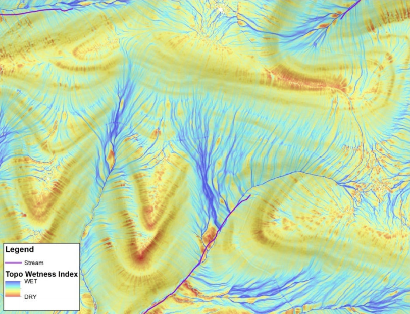
This combination of large contributing area and low slope is considered one of the most important predictors of where saturation is likely to occur within a watershed. The formula ln(a/tan B), where a is the upslope contributing area and B (beta) is the local slope angle is called the topographic wetness index. The topographic wetness index underlies the widely used TOPMODEL numerical watershed model and predicts depth to the water table in order to generate overland flow.
Example of the topographic wetness index variation for a small area within the Susquehanna River basin. From Zimmerman and Shallenberger (2016).
Soils matter in a lot of ways. Infiltration capacity is important for determining whether infiltration-excess overland flow will occur. Hydraulic conductivity (and its profile with depth) determines how easily water moves through the soil – and therefore how quickly downslope drainage can occur. Depth is important for determining how likely saturation is to occur (deep, high conductivity soils require a lot of water in order to achieve saturation). You won’t be surprised to learn that soil properties have been used as strong predictors of water transit times
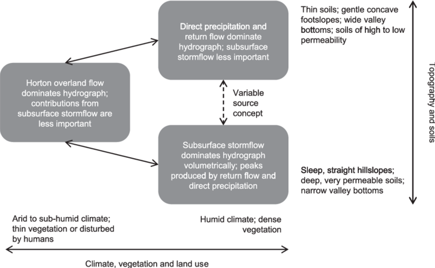
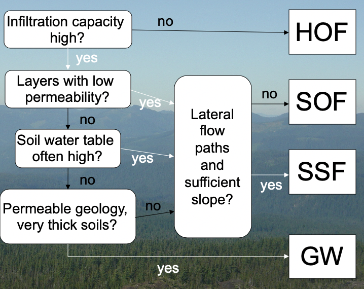
I find this flow chart helpful in thinking about the role of soils and topography in controlling streamflow generation processes.
HOF is Hortonian (or infiltration excess overland flow). SOF is saturation overland flow. SSF is subsurface stormflow and GW is groundwater. This diagram is simplified from one presented in Schmocker-Fackel et al. (2007).
Geology
The astute geologists among you will be noting that topography and soils are both, in large part, a function of a watershed’s geologic history. Some even say that geology is destiny.
Below the soil, the hydraulic conductivity of the parent material controls how much deep percolation and groundwater flow can occur. If the bedrock has low hydraulic conductivity, then subsurface stormflow can be set up. However, even in low conductivity rocks, fractures can become important flowpaths for groundwater movement that sustain baseflow in streams. If the bedrock or other parent material has very high hydraulic conductivity (like alluvium, limestone, and basalt do), aquifers may feed streams and rivers, even in the near-absence of other flow generating mechanisms. Such groundwater-dominated streams often have very steady baseflow and very muted stormflow responses to precipitation compared to streams fed by other subsurface stormflow, saturation overland flow, or infiltration excess overland flow.
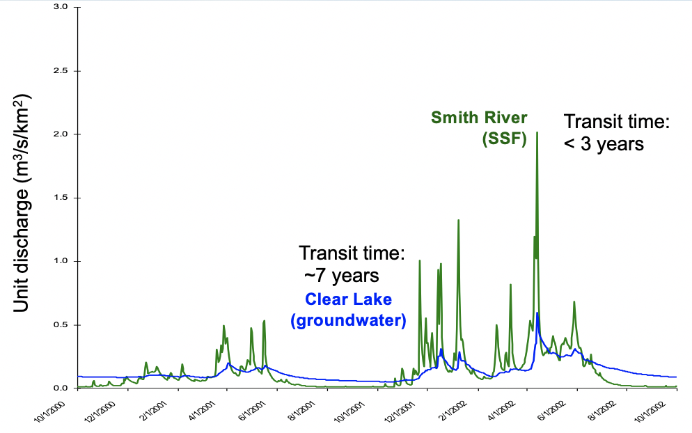
The peculiar hydrology of groundwater-dominated streams and how their flow was regulated by geology was the subject of my PhD. I studied streams in the central Oregon High Cascades, where winter snow and rain recharge aquifers in Quaternary basalt lavas. These basalts have very high hydraulic conductivity and their groundwater feeds huge springs and supports beautiful rivers. Just to the west of the High Cascades, the Western Cascades has Neogene volcanic rocks that with lower hydraulic conductivity. In the Western Cascades landscapes, subsurface stormflow dominates and the hydrographs are much more responsive to winter storms and summer droughts.
Two streams with adjacent watersheds, similar vegetation and climate, and contrasting geologic history end up with very different hydrographs and transit times.
We’ve already alluded to the importance of human activities in altering hydrology and flow generation. Urban areas are characterized by impervious surfaces (pavement and rooftops) that prevent infiltration and promote infiltration-excess overland flow. Mining, military and industrial activities denude the landscape of vegetation and compact the soils, resulting in a greater propensity for overland flow. Forest harvest reduces interception, and can compact the soil. Agricultural practices can radically alter the soil profile, especially when plowing is involved. A compacted layer below the plowing depth can lead to perched saturated zones that can reach the land surface and generate overland flow. And grazing animals compact the soil profile and promote infiltration excess overland flow. Tile drains are giant subsurface preferential flowpaths, just like storm sewers. Basically everything that humans does tends to increase the propensity for rapid drainage of water from the landscape, whether that occurs via overland flow or through anthropogenic macropores (i.e., pipes).
(And that’s what connects what I research now with urban hydrology to the volcano hydrology I used to do…I’m interested in how water moves through landscapes and what that means for streams.)