An appropriate demonstration on this Earth Day of the power of our planet. But it’s also notable that, except for the last few seconds, which show that this footage comes courtesy of some climbers who were (fortunately) traversing the opposite side of the valley, there was not a human or building in sight. This is a striking contrast with the normal lens through which we view events like this, which is in terms of how they affect us, and our civilisation*. The pictures coming out Sichuan Province in China, in the wake of the weekend’s magnitude 6.6 earthquake, illustrate this quite well.
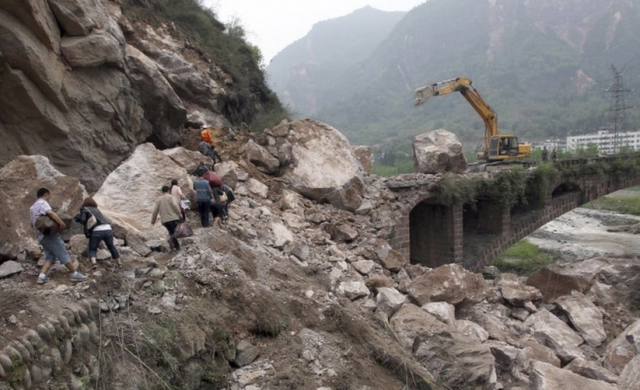
A landslide blocking a road and bridge in Sichuan province, China. Source: BBC.
This tendency is perfectly understandable, but it does speak to a certain hubris on our part. The (French) commentary to that avalanche video mentions that this is just a normal part of spring in the Alps, as the snowpack warms up. Earthquakes and volcanoes, storms and floods, landslides and avalanches; all of these ‘hazards’ are in a sense, just the earth doing its thing, and have been happening for hundreds of millions of years before humanity was around to menace. Even now, they only become disasters when we get in the way. But we tend to think of it in terms of nature intruding on us, rather than the other way around.
It’s a very strange way of looking at things, really: we create our little civilised bubbles on an active and vibrant planet, and then manage to be continually surprised when reality decides to pop them. As Terry Pratchett’s anthropomorphic personification of Death comments in The Hogfather,
STARS EXPLODE, WORLDS COLLIDE, THERE’S HARDLY ANYWHERE IN THE UNIVERSE WHERE HUMANS CAN LIVE WITHOUT BEING FROZEN OR FRIED, AND YET YOU BELIEVE THAT A…BED IS A NORMAL THING. IT IS A MOST AMAZING TALENT.
A similar sentiment can be found in New Zealand nowadays, as they are forced into an uncomfortable confrontation with the true dangers in their beautiful yet dangerous homeland:
“If you’re not on a fault zone, a volcanically active zone, or a tsunami zone, you’re probably in a valley that’s prone to flooding or having things tumble down the hills towards you.”
I sometimes wonder if our feet-dragging on the issue of climate change doesn’t partly stem from the same detached attitude: we just can’t understand that what we do in our homes and cities can affect the world out there. So my thought for Earth Day is this: if we want to have a long-term future on this planet, we’re going to have to learn that our only hope of rolling with the planetary punches is not a doomed quest to set ourselves outside of nature, but to embrace it, and understand it, and allow ourselves to be shaped by it.
*I think this might actually be changing though, as video cameras in phones, and the ability to easily upload footage, become more widespread.
On Saturday morning local time (Friday evening for us in the USA), a magnitude 6.6 earthquake shook up Sichuan province in western China, about 35 km north of the closest city, Ya’an, and 115km west of the provincial capital Chengdu. Its shallow depth (about 12 km, according the USGS), meant strong shaking above the rupture; so far more than 150 deaths have been reported, with hundreds more injured. This BBC report includes footage of the shaking and collapsed buildings.
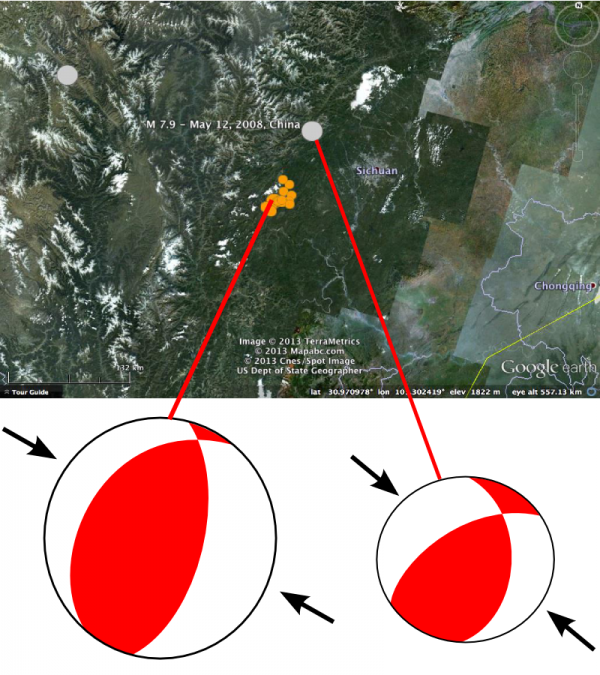
This is the same region that was shaken by the much larger magnitude 7.9 Wenchuan earthquake on May 12 2008, resulting in tens of thousands of deaths; in fact, that rupture was less than 100 km north-northeast of this latest one. When added to the fact that the focal mechanisms for both earthquakes are also very similar, indicating WNW-ESE compression on a NNE-SSW trending fault, this relative location makes it likely that we are seeing a further rupture of the same fault system that failed in the Wenchuan earthquake – either an adjacent segment of the same fault, or another, similarly oriented fault in the same thrust system.
Location and focal mechanism for M 6.6 earthquake on 20th April 2013 in Sichuan Province China (orange dots include first 12 hours of aftershocks) and the May 2008 M 7.9 Wenchuan earthquake (grey dot). Data from USGS.
The ultimate cause of this earthquake is the continental collision that has produced the Himalayan mountains to the east. As India continues to push into Asia, some of the Asian crust is pushed out of the way upwards, creating the looming heights of the Himalayas and the Tibetan plateau; but some is also being pushed out of the way sideways in the direction of China. The Longmenshan mountains, where all this seismicity is occurring, mark a place where there is a particularly strong bit of Chinese crust – the Sichuan Basin – standing against this tectonic invasion, forcing the eastwards migrating crust to be thrust over it. For more details and some nice explanatory figures, check out Kim Hannula’s post on the tectonics of the 2008 earthquake.
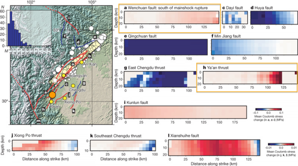
The other question to consider is whether the Wenchuan quake was an influence om the timing and location of this latest rupture. In a discussion on Twitter Eric Fielding pointed me to this July 2008 paper by Parsons et al. that calculated the permanent stress changes on neighbouring and nearby fault segments induced by the Wenchuan rupture: they concluded that it caused the stress to increase on both the southern continuation of the Wenchuan Fault itself, and the parallel Ya’an Thrust that may be a better candidate for the source of the current shaking.
A tectonic map of the Longmenshan thrust system. The accompanying cross-sections of other faults in the area show modelled increases (red) and decreases (blue) in permanent stress resulting from the 2008 M 7.9 Wenchuan earthquake (white star). Orange boxes highlight the southern segment of the Wenchuan Fault and the Ya’an thrust – both possible sources of the latest quake, whose rough location is shown by the orange circle. Modified from Parsons et al., 2008
This makes it possible that events in 2008 did indeed prime the pump for an earthquake 5 years later, in the sense that it added a little bit of extra stress onto the fault that ruptured last night, and caused it to fail earlier than it would have otherwise. However, the reason that there was a stressed fault ready to fail in the first place is the wider tectonic forces associated with the Himalayan collision.
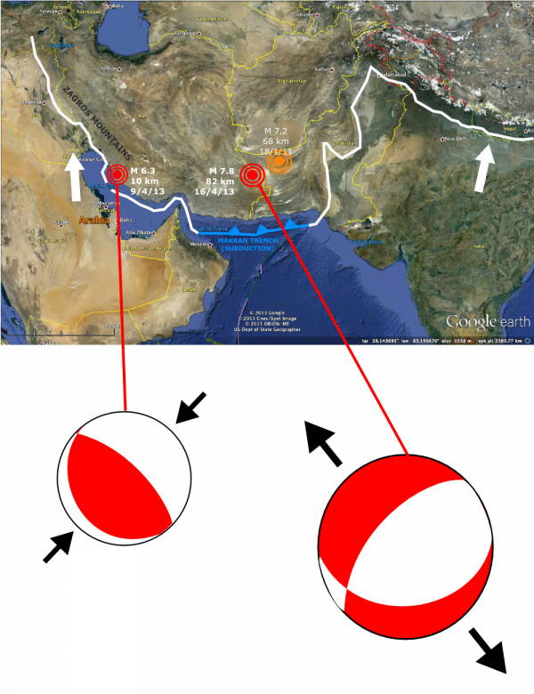
Squashed and squeezed between the Eurasian continent to the north and the northward-moving Arabian plate to the south, it is no surprise that Iran is a seismically active country, and in the past week it has been living up to expectations. Last Tuesday, a magnitude 6.3 earthquake at 10 km depth shook the western Bushehr region on the coast of the Persian Gulf; this Tuesday, a much larger magnitude 7.8 rupture occurred in the western province of Sistan Baluchistan, near the border with Pakistan.
Location and focal mechanisms of the two recent large earthquakes in Iran. Data from the USGS.
The USGS originally reported the rupture depth for this week’s quake as 15 km, but as more data was analysed the estimate became much deeper, around 80 km depth (other solutions suggest it’s closer to 50 km). This meant that although this quake was powerful enough to shake buildings from Oman to India, the strength of the shaking immediately above the rupture was far less powerful than was originally feared. Although the mud brick buildings common in this region are not particularly resilient to earthquakes, the largest death toll reported so far is 34 people across the border in Pakistan.
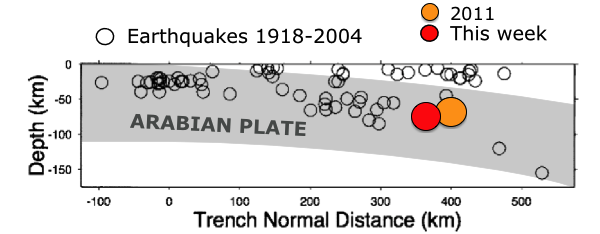
The map above shows that both these earthquakes are associated with the collision of the Arabian and Eurasian plates, although there is a transition from a full-on continental collision in the west to a subduction zone (the Makran Trench in the east). However, the focal mechanisms for these two earthquakes are very different, last Tuesday’s M 6.3 indicating northeast-southwest compression and this Tuesday’s M 7.8 indicating northeast-southwest extension. The former is much more in keeping with what you’d expect at a collisional plate boundary than the latter, at least until you remember that the depth of the rupture makes it much more likely to have occurred in the subducted Arabian slab that must exist underneath eastern Iran and western Pakistan, rather than the folded and crumpled Eurasian plate we see on the surface. In fact, as I’ve also marked on the map above, in January 2011 a magnitude 7.2 earthquake with a very similar depth and extensional focal mechanism occurred around 250 km to the northwest of this week’s rupture in western Pakistan. The plot below, modified from Engdahl et al. (2006) shows both of these earthquakes fall within the projected confines of the subducted Arabian plate; the extensional focal mechanisms are probably therefore caused by either the pull of the down-dip slab, or some sort of plate bending effect.
Rough shape of the subducting Arabian plate (shading added by me) based on the earthquake locations of Enghdal et al. (2006), with approximate locations of this week’s M 7.8 earthquake and the very similar M 7.2 event in western Pakistan, Jan 2011.
As I noted in 2011, the northwest-southeast axis of extension is considerably rotated from the north-south axis you would predict for either ‘slab-pull’ on, or bending of, a north-dipping slab, so some other forces may be at play; perhaps the faster collision of India to the east that forms the Himalayas is forcing some kind of lateral buckling of the Arabian slab.
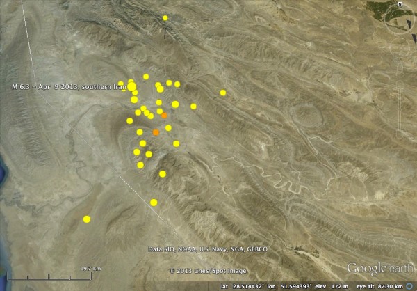
I was also quite interested in last week’s magnitude 6.3, because it was located in the Zagros mountains: the main shock and aftershocks are located right amidst some of the beautiful folds for which the region is famous, traced out in aerial view by resistant limestone ridges.
Location of last week’s M 6.3 in the Zagros mountains, with aftershocks and pretty, pretty folds. Data from USGS.
The Zagros region is also an example of thin-skinned thrusting, where a layer of weak rock – in this case a Cambrian evaporite – acts as a detachment, or décollement, which isolates folding and thrusting in the surface layers from the deeper parts of the crust. As such, you would expect seismicity in this area to be located on this decollement, or on thrust splays propagating up from it. A nice cross section across this region can be found in McQuarrie (2004), and indicates that the 10 km depth of the rupture is close to the decollement depth, but combining the information from the focal mechanism with this section suggests the rupture was on a NE-dipping splay fault. McQuarrie also suggests that most of the faults are associated with the cores of the folds observed at the surface, although it is hard to clearly see this from the aftershock pattern.
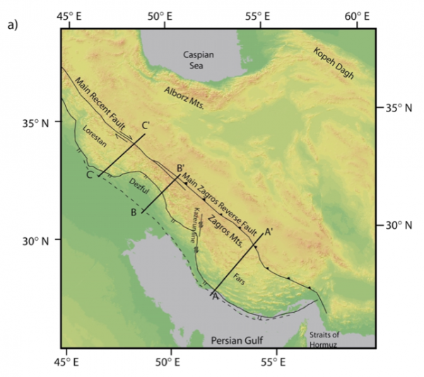
Map of Zagros Mountains. Cross-section A-A' is reproduced below. From McQuarrie(2004).
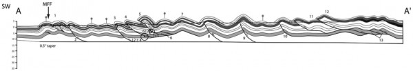
Balanced cross-section through Zagros fold belt in the same region as last week’s M 6.3 Earthquake. From McQuarrie (2004).
So it seems that Iran’s seismic week encompassed both shallow and deep collisional processes, on opposite sides of the country. And tempting as it is to look for some deeper reason for both of these earthquakes occurring within a week of each other, the Bushehr earthquake last week was probably too small and far away to have had any influence on the timing of this week’s rupture.
It’s been another month of fascinating scientific adventures for your resident hydrologist.
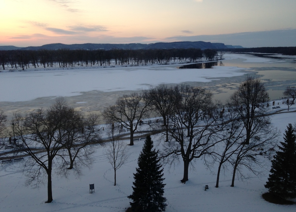
It all began at the end of February, when I travelled to La Crosse, Wisconsin to the Upper Midwest Stream Restoration Symposium, which was a really stimulating and vital mix of academics, consultants, and government folks all interested in improving the state of the science and practice of stream restoration. I gave a talk on Evaluating the success of urban stream restoration in an ecosystem services context, which was my first time talking about some hot-off-the-presses UNCC graduate student research, and I learned a lot from the other speakers and poster presenters. While the conference was incredibly stimulating, travel delays due to bad weather on both ends of my trip made for a somewhat grumpy Anne (nobody really wants to spend their birthday stuck in a blizzard in O’Hare), so I’ll be thinking carefully about how to plan my travel to the Upper Midwest during future winters. Nonetheless, the view from the conference venue was phenomenal.
View of the Mississippi River from the Upper Midwest Stream Restoration Symposium in La Crosse, WI. Not shown: bald eagles that frequent the open water patches of the river.
March proper saw me give variations of the restoration talk two other times. On the 15th, I gave it as the seminar for Kent State’s Biological Sciences department, and on the 26th, I gave it at the North Dakota State University Department of Geosciences (more about that trip below). In between, I gave a seminar on the co-evolution of hydrology and topography to the Geology Department at Denison University in Granville, Ohio. Students in that department had just returned from a trip to Hawaii, and a very memorable dialogue occured in the midst of me talking about the High Cascades:
“You’ve seen a young lava flow. What would happen if you poured a bottle of water on it?” “It would steam!” “Not that young!”
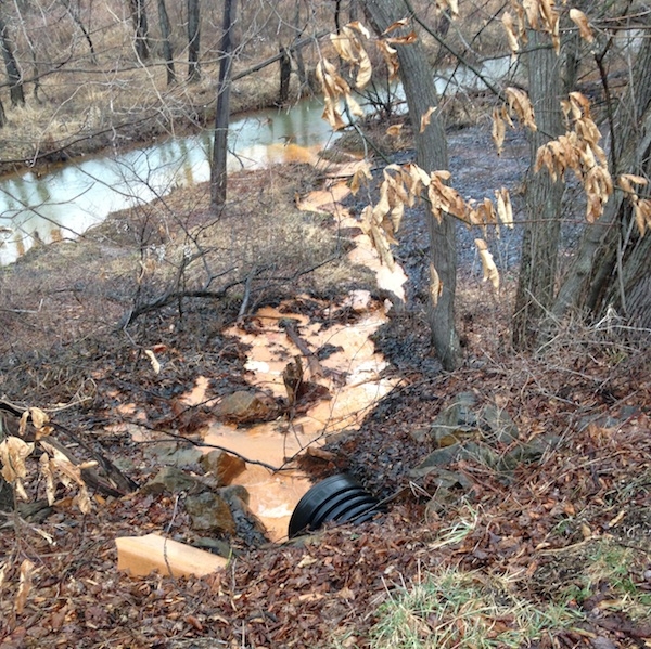
Closer to home I also hosted a couple of prospective graduate students, helped interview candidates for a faculty position in our department, and went with a colleague to visit an acid mine drainage site about an hour to the south of Kent. In one fairly small watershed, we were able to tour a number of different remediated and unremediated sites, and it certainly lent a whole different perspective to the ideas of stream restoration and constructed wetlands to look at a landscape irrevocably scarred by mining activities.
Unremediated acid mine drainage flow directly into Huff Run. The orange is iron precipitate.
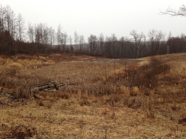
Constructed wetland as the second stage of acid mine drainage remediation in the Huff Run watershed.
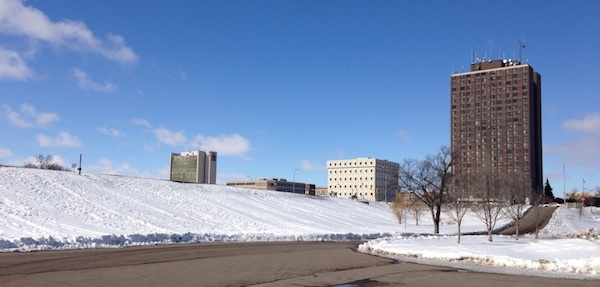
At the end of the month, we finally got our turn for spring break. I ended up with a somewhat epic combination of mounds of work and a big trip to take, possibly the worst combination of the untenured and tenured professor spring break stereotypes (see this PhD comics strip). The first half of the week, I spent in Fargo, North Dakota, home to the famously flood-prone Red River of the North. (I’ve blogged before about why the river so often produces expansive floods.) It was truly fascinating to put my feet on the ground in a place that I’ve read about and watched from afar for years. And my visit was made all the more interesting by my host and guide, Dr. Stephanie Day, a geomorphologist newly at NDSU and who may well unravel some of the Red’s geomorphological peculiarities.
Stephanie Day, Assistant Professor of Geosciences at North Dakota State University beside the Red River in Moorhead Minnesota. The flat surface in the background is the approximate elevation of the land for miles around.
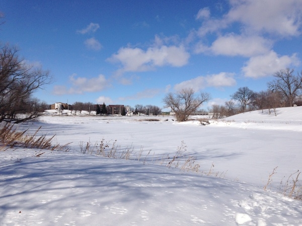
Looking towards downtown Fargo, ND from the river side of the levee.
River’s edge view looking towards downtown Fargo. Snow well over knee deep here on 25 March, by my measurements. As all that snow starts to melt, the water will rise.
There’s a pretty good chance we’ll see a major flood on the Red River later this spring, as the >24″ of snow melts out of the watershed, runs off over frozen ground, and enters the northward flowing river. The Fargo Flood page is the place to go to follow the action, and you can count on updates (and more pictures) here as events unfold.
The latter half of my spring break saw me diagonal across the state of Minnesota to my beloved Driftless Area, back across the Mississippi River, and into the state of Wisconsin. I saw my family, finished paper revisions, and wrote part of a grant proposal. Then I flew home, with nary a weather delay in sight.
If March was a tight, recursive meander of talks and trips to the Upper Midwest, then April promises to be a bit anastomosing with lots of different threads woven together to make another month of scientific delight.
Combined sewers are pipes that catch both sewage and stormwater and route it to a waste water treatment plant. In dry weather, it’s all sewage in the pipes. In small rain storms, the pipes carry sewage mixed with stormwater and it all goes to the wastewater treatment plant to get cleaned up and returned to a stream or lake. The origins of combined sewers predate waste water treatment, when there was little distinction between stormwater and sewage and stream and city dwellers just wanted the foul-smelling, disease-festering stuff out of their way as soon as possible. Later, engineers and public health folks added the crucial waste water treatment plant step to the system but the sewers remained combined. Combined sewers were common until the early 20th century, so over 772 communities in the US, mostly in the Northeast and Great Lakes regions have combined sewers, as shown on this map from the US EPA:
US EPA map of Combined Sewers. Click for source.
Most of the time, combined sewers route all of the water to the waste water treatment plant, and all is relatively well. But in large storms, the volume of stormwater and sewage can overwhelm the waste water treatment capacity. If the volume of water was too much to treat, you can imagine the pipes starting to fill up with sewage. If there were no “pressure release valve” on the system, urban dwellers in combined sewer cities would see the sewage/stormwater cocktail start to back up into their basements, sinks, … and, you get the picture. Fortunately for those city residents, there is a “pressure release valve in the system,” but it’s a solution that creates more problems downstream, literally. When flows in the combined sewers are too great to be treated, the sewage/stormwater cocktail overflows out of the pipe network and into local streams. Then you’ve got raw sewage in your stream and that’s not pretty, or healthy, or environmentally friendly. This is the infamous combined sewer overflow or “CSO.”
US EPA diagram of a combined sewer in dry and wet weather. From U.S. Environmental Protection Agency, Washington, D.C. “Report to Congress: Impacts and Control of CSOs and SSOs.” Document No. EPA 833-R-04-001 found on Wikimedia commons. Click for source.
Here’s a Northeast Ohio Regional Sewer District video explaining combined sewers and touting their treatment system:
Under the Clean Water Act, cities and sewer districts can be required to bring their raw sewage discharges down to acceptable levels by reducing the frequency and magnitude of combined sewer overflows (CSOs). Right now, Cleveland, the District of Columbia, Philadelphia, and other cities are under mandate to reduce their CSO discharges. This is a big, expensive undertaking because we’re talking about billions of gallons of overflows each year and thousands of miles of combined pipe network underneath the city. Big problems require big solutions, so how are the cities dealing with their CSO problem? It turns out that they are taking a range of different approaches.
In Cleveland, waste water treatment and stormwater are managed by the Northeast Ohio Regional Sewer District (NEORSD). Their “consent decree” with the EPA was filed in July 2011, and according to that decree, they have 25 years to reduce CSO volumes by 90%. That’s taking the CSOs from 4.5 billion gallons per year to the still non-trivial 494 million gallons per year. If they meet that goal, 98% of all wet weather flows will be treated before being released to a stream. The price tag for this ambitious project is $3 billion, and it has been termed “Project Clean Lake” in homage to Cleveland’s Lake Erie shoreline. a source of regional pride.
How is NEORSD planning to reduce CSOs? With a lot of digging. Most of the money and effort is being spent on “gray infrastructure” – big engineering projects. BIG engineering projects. NEORSD is boring 7 tunnels, each 2-5 miles long, up to 24 feet in diameter, and up to 300 feet below the ground or lake bottom. These tunnels will intercept the combine sewers before they overflow and store the water until the treatment plants have capacity to treat it.
The 7 future storage tunnels of Cleveland’s combined sewers. Image courtesy NEORSD. Click for larger.
This is a massive undertaking, and it’s just getting started. The videos below show the first tunnel boring machine arriving in Cleveland and a tour of the tunnel first tunnel to begin construction. You can follow the progress of the tunnel boring on the NEORSD blog.
But it’s not just tunnels, NEORSD is also enhancing their wastewater treatment capacity and spending $42 million on green infrastructure. Green infrastructure is defined as “a range of stormwater control measures that use plant/soil systems, permeable pavement, or stormwater harvest and reuse, to store, infiltrate, or evapotranspirate stormwater.” These can include things like green roofs, green streets, bioretention swales, and other projects. The goal is control 44 million gallons of would-be stormwater using green infrastructure, with projects completed in the next 8 years. Those numbers are nothing to sneer at it, but it’s 1% of the current combined sewer overflow volume and 1.5% of the budget. The fact that the budget % is bigger than the volume percent may hint at why green infrastructure isn’t being used more broadly in Cleveland.
Washington DC is taking a somewhat different approach than Cleveland. One-third of DC is served by combined sewers, and they are spending $2.6 billion over 25 years to reduce their overflow problem, which is currently about 2.5 billion gallons per year. DC Water has nicknamed their CSO program the “Clean Rivers Project.” Like Cleveland, they are also building large storage tunnels, improving their waste water treatment plants, and rehabilitating pumping stations. Unlike Cleveland, DC will actually be separating the sewers in some areas, sending sewage and stormwater down different pipes from each other. In DC, green infrastructure seems to get only a rhetorical nod, rather than a significant component of the budget. Their plan says they will “advocate implementation of Low Impact Development,” but they’ve only budgeted $3 million for it, a mere 0.1% of their overall project cost. However, they do have the world’s best explainer video.
Philadelphia is taking a radically different approach. Like Cleveland and DC, their price tag comes out to about $3 billion over 25 years. However, in Philadelphia it’s a “Green City, Clean Waters” program and green infrastructure steals the show. Philadelphia’s goal is to “reduce reliance on construction of additional underground infrastructure” by pushing extensive green infrastructure throughout the city. In other words, they don’t want to dig tunnels. Instead, they want to green acres:
Each Greened Acre represents an acre of impervious cover within the combined sewer service area that has at least the first inch of runoff managed by stormwater infrastructure. This includes the area of the stormwater management feature itself and the area that drains to it. One acre receives one million gallons of rainfall each year. Today, if the land is impervious, it all runs off into the sewer and becomes polluted. A Greened Acre will stop 80–90% of this pollution from occurring.
Philadelphia’s rationale for making green infrastructure their big push centers around social and economic benefits to come and their historic heritage as a park city. Their video is all about people, not all about pipes:
Philadelphia’s vision is the most radical departure from a traditional “grey infrastructure” approach like that pursued in Cleveland, DC and other cities. There’s certainly an aesthetic and emotional appeal behind greening a city and its stormwater. This is the way many people want to move urban hydrology in the 21st century, integrating the built and natural environment more closely than we’ve done in the past. But it will be interesting to watch where Philadelphia succeeds and if and where it fails, as the fully green infrastructure approach could be seen as much riskier than a traditional engineering-driven approach. Fortunately, EPA is devoting some funding to research on the effectiveness of Philadelphia’s project. I won’t be doing that work directly, but I will be following it closely and think it would be fascinating to put together a more rigorous multi-city analysis of approaches and outcomes.
More broadly, the combined sewer overflow problem is a fantastic example of how our environmental and societal choices are constrained by decisions made in the past. No one today would build a combined sewer, but yet millions of people live in cities served by them, thousands of engineers, scientists, and sewer district workers work with them, and billions of dollars are being spent trying to mitigate the problems they cause. We can’t just rebuild cities from the underground up, so we have to work with what we’ve inherited and try to make decisions that won’t cause consternation for future generations.
Note: This blog post is adapted from the lecture I gave today in Urban Hydrology. If I’ve gotten anything wrong or missed an important point, please let me know and I’ll try to make it better for current and future students.