Highly Allochthonous | NEWS & COMMENTARY FROM THE WORLD OF GEOLOGY & EARTH SCIENCE

4 index fossils

Posted on December 28, 2009 by Chris Rowan

On the 4th day of Christmas my true love sent to me: 4 index fossils…

Sometimes when you are studying a geological sequence, the most basic problem you need to address is establishing a reliable chronology – not just how old it is, but how much geological time is spanned not only by the whole sequence, but by specific beds or horizons within it. Only then can you start to examine the possible rates of environmental changes, and correlate them to changes in other sequences in the same region, or around the world. A good chronology needs as many well-dated ‘tie-points’ as possible; dating volcanic material is all well and good, but if your section contains one datable volcanic ash at the top, and all the interesting stuff is happening at the bottom, it’s not particularly helpful.
This is where biostratigraphy comes into its own. Particularly in marine sequences, fossils are much more abundant than datable horizons, and there exist several groups of organisms that provide highly useful and precise time stamps for the rocks they are found within, because they combine a wide geographic range (allowing regional or even global correlations) with fast rates of evolution, such that within quite a short time (geologically – it’s still usually at least a million years or two) some easily distinguishable physical characteristic changes markedly enough that they are classified as another species. These index fossils are therefore wonderful tools for filling in the chronological gaps.
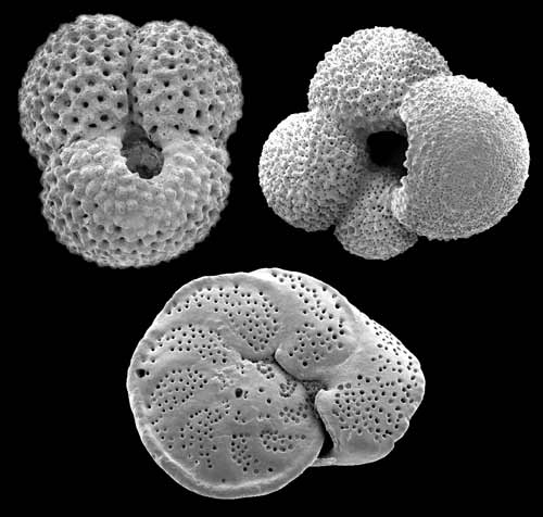
Different index fossils are useful for different periods of earth’s history. One of the more common groups used when studying sediment cores brought up from the seabed (which range in age from 180 million years to essentially modern), are foraminefera, single-celled plankton with hard calcareous shells, and a very large diversity of morphological forms

Source

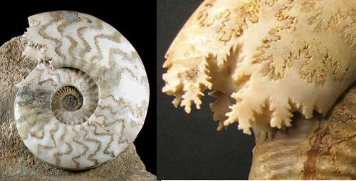
Going further back in geological time, one of everyone’s favourite fossils, the Ammonoids, are extremely useful index fossils for Late Paleozoic and Mesozoic sequences, such as southern England’s Jurassic Coast. Many different species are easily identified by the different, and often highly intricate. patterns of their sutures – the lines where the walls of the chambers in their shells connect to the outer shell.

Source 1, 2

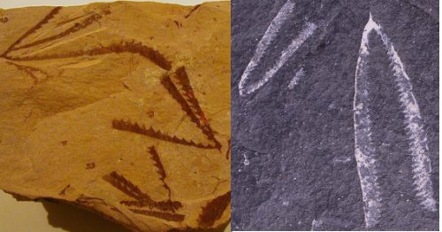
For the early Palaeozoic, graptolites – free-floating colonial organisms that populated the world’s oceans in the Ordovician and Silurian periods, between about 490 and 370 million years ago – are firm favourites.

Source 1, 2

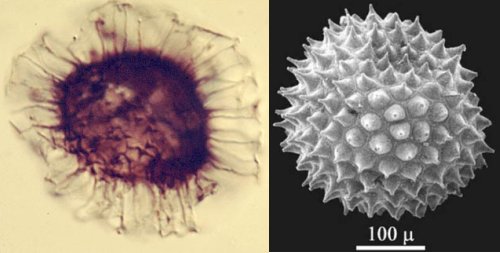
Even generally fossil poor Precambrian rocks may contain potential index fossils, in the form of Acritarchs. This is not a ‘natural’ fossil group, in that everything that is identified as an acritarch is not necessarily closely related in evolutionary terms; a good working definition of them would be ‘organically walled microfossil that we’ve found but can’t really identify, and the ‘Acritarch’ actually means ‘of uncertain origin’. Palaeontologists’ best guess is that they’re probably mainly algal cysts. However, even if this group does contain lots of different ancient single-celled organisms lumped under the same banner, their fossil record stretches back into the Precambrian (the oldest known lived more than 2 billion years ago), possibly allowing for some biostratigraphic correlation between sequences from a time otherwise distinctly lacking in a fossil record, including the Neoproterozoic where I’m currently working.

Source 1, 2

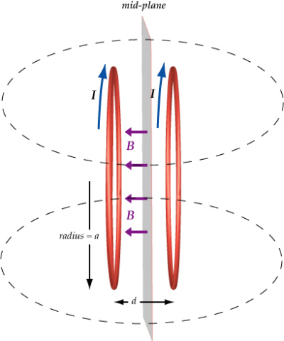
…3 Helmholtz coils,

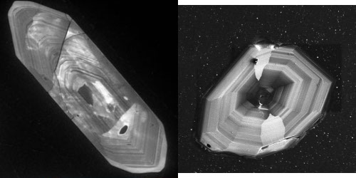
2 concordant zircons,

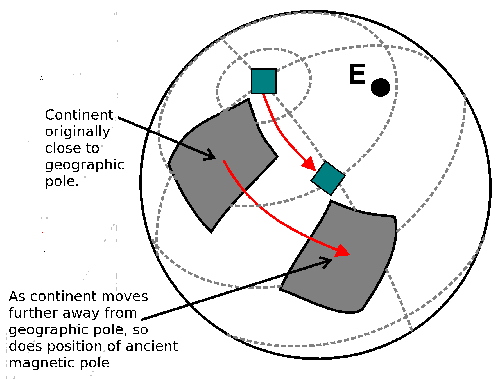
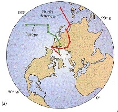
and an APWP.

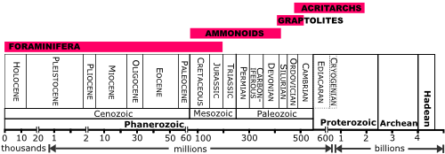
Useful time ranges for index fossils mentioned in this entry

Categories: fossils, geology

3 Helmholtz coils

Posted on December 27, 2009 by Chris Rowan

On the 3rd day of Christmas my true love sent to me: 3 Helmholtz coils…

If you’re trying to measure the often rather weak magnetisation of rock sample, the last thing you need is other magnetic fields invading your measurement space and mucking up your readings. To avoid this, the magnetometer is placed in a magnetically shielded space. One method of doing this is to build a shielded room with walls made out of a material with high magnetic permeability, such as Mu-metal or transformer steel, that absorbs most of the magnetic flux before it encroaches inside. However, cost or space issues sometimes make this impractical.
An alternative is to generate your own magnetic field around the magnetometer, such that it cancels out the ambient field in your lab. For this to be effective, you need to have a set-up that will generate a uniform cancellation field within a volume large enough to fit your measuring equipment, which means that you employ paired Helmoltz coils. With the right separation, if you run a current around the coils a uniform axial magnetic field is created in the region between the coils.

image source

In order to cancel out the ambient magnetic field completely, therefore, you need three pairs of Helmholtz coils, nested within and oriented perpendicular to each other. If you’re feeling fancy, you can even set up an active control system that will automatically account for changes in the ambient field: both natural changes due magnetic fields of the sun and moon, and the solar wind, interacting with Earth’s magnetosphere, and unnatural ones due to lorries parking outside your lab, cars moving past, or those crazy physicists down the hall.

Helmholtz cage.JPG
image source

With such a control system in place, most of the time you can reduce the magnetic field inside the coils from around 50,000 nano-tesla to less than 50 nano-tesla, which is just as good as being inside a mu-metal box. However, it is a slightly less stable low field environment, because rapid fluctuations in the field will sometimes occur too fast to be corrected for. My last two laboratories had magnetometers in shielded rooms, whilst my current laboratory in Edinburgh has a set of Helmholtz coils; so over the next few months I’ll be able to check their relative effectiveness for myself.

…2 concordant zircons,

and an APWP.

Categories: geology, geophysics, palaeomagic

2 concordant zircons

Posted on December 26, 2009 by Chris Rowan

On the 2nd day of Christmas my true love sent to me: 2 concordant zircons…

If you want to accurately date a rock, you really want to grind it up and extract some grains of zircon. This mineral has several useful properties: it is very hard and chemically inert, even at quite high temperatures, so will survive relatively intact even if the rest of the rock it is surrounded by is extremely squeezed, squashed and metamorphosed.

image source 1, 2

In addition, zircon’s crystal structure allows lots of uranium to be trapped within a grain when it forms, but virtually no lead. This doesn’t mean that you don’t find any lead within zircons if you chemically analyse them – you do. But this lead was produced within the crystal after it formed, by the radioactive decay of uranium. In fact, two different decay processes are at work: uranium 238 decays to lead 206, uranium 235 decays to lead 207. Therefore you have two ways of getting a radiometric age for the zircon: you can measure the ratio of uranium 238 to lead 206, or you can measure the ratio of uranium 235 to lead 207. This means that zircons have a built in cross-check: if you calculate the age using both of these ratios, and they are the same within error, the age is said to be concordant, and you can have more confidence that the age you have determined reflects the original age of formation (a resetting event would affect the different ratios to a different degree, and result in discordant ages).
We’re currently trying to extract some zircons – or baddeleyites, which are similarly useful for dating but more common in mafic rocks than zircons sometimes are – from the dykes I sampled in Oman last year. Of course, I could probably do with more than two, but two would be a start!

…and an APWP.

Categories: geology, rocks & minerals

An APWP

Posted on December 25, 2009 by Chris Rowan

On the 1st day of Christmas my true love sent to me: an APWP

APWP stands for ‘apparent polar wander path’. The remanent magnetisation imprinted on a rock as it forms points towards the magnetic pole, and from its direction you can calculate where, geographically, the pole that the rock ‘saw’ falls on the Earth’s surface. Often, the pole position you calculate from the magnetisation directions of older rocks is some distance from the current geographic poles. It would have plotted there just after the rock formed, but after millions of years of plate motion, the continent it formed on is now at a different longitude and latitude, and hence a different distance from the geographic poles, than it was long ago. This phenomenon is called ‘apparent polar wander’, because it looks like the magnetic pole has moved with respect to the Earth’s surface, although in fact it is the Earth’s surface moving relative to the Earth’s magnetic pole.

A remanent magnetic pole which originally plots at the geographic pole will plot away from it after millions of years of plate motion

By plotting the magnetic poles for a sequence of rocks formed over tens or hundreds of million years, you get a record of continental motion over geological time: an apparent polar wander path or APWP. And if you can obtain APWPs for two different continents spanning a similar age range, you can get an idea of differential motions between them. For example, the APWPs for Europe and North America have a very similar shape between about 350 million and 100 million years ago (the sections of the lines furthest from the current geographic pole in the figure below), when they were both part of the supercontinent Pangaea and henced moved as one; indeed, if you close up the Atlantic Ocean that now separates them, the two paths will overlap.

Apparent Polar Wander Paths for North America and Europe since the Permian.

The project I’m working on at the moment is currently trying to generate APWPs for the different continents in an earlier time period, between 1000 and 500 million years ago. So this palaeomagician would love an APWP as a Christmas gift – although any sensible true love would certainly point out that I’m the one being paid to produce such a thing…
Note: this series is intended to be a light-hearted , and mildly educational, list of useful geological things. Hopefully, you don’t get too bored of this bit of seasonal whimsy before 12th night – if indeed you bother to check your RSS feeds before then!

Categories: geology, palaeomagic

Here comes the sun…

Posted on December 21, 2009 by Anne Jefferson

A post by Anne Jefferson The Earth’s axis has a 23.44^o obliquity or tilt to it. As the Earth revolves around the Sun over the course of a year, the axial tilt means that different parts of the Earth’s surface receive direct sunlight at different times of the year. And it’s this receipt of varying intensities of solar radiation that drives temperature differences, and hence seasonality.
Today is a solstice, illustrated by the image on the far right below. Today is the day of the year when the Northern Hemisphere is tilted farthest away from the sun and the Southern Hemisphere is tilted most towards the sun. For those of us in the Northern Hemisphere, it’s our shortest day of the year and the sun never gets very high in the sky, even at noon. In fact, the word solstice has a Latin origin in the word solstitium, where “sol” means sun and “stitium” means stoppage. and for several days around the solstice this noontime elevation appears to be the same – hence the stoppage. Today, the noontime sun appears directly overhead along the Tropic of Capricorn, 23.44^o S.

Figure 1. Earth at the solstices and equinoxes, as seen from the north. Source: Wikimedia.
The precise moment of the solstice occurs at 17:47 UTC (12:47 pm Eastern Standard Time). We’ll have another solstice (image on far left) on 21 June 2010 at 11:28 UTC ( 7:28 am Eastern Daylight Time). Over the course of the Earth’s trip around the Sun there will be two moments when everybody is getting their fair share of sunlight – the equinoxes. In 2010, they’ll occur on 20 March 2010 at 17:32 UTC and 23 September 3:09 UTC (22 September 11:09 pm EDT).
Earth’s tilt also varies over geologic time. It has a ~41-thousand year cycle, and right now we’re at about the middle of the range in variation of axial tilt. As tilt increases, seasonal contrasts over much of the world increase, but it is decreased axial tilt is tied with the onset of continental glaciation. That’s because at high latitudes, when tilt is low, summers are even cooler, and more snow persists through the summer. That surviving snow forms the nucleus of glacial ice caps. We’re currently on the decreasing limb of the obliquity cycle, but based on past occurrence of continental glaciations, the onset of another one is going to require not just less obliquity, but also the right eccentricty and precession in the Earth’s orbital parameters and controlling greenhouse gas emissions.

Figure 2: Last seen at Clastic Detritus in 2007, original created by Slumbering Lungfish.