
The big picture
Now that you’ve learned all about the four different ways to generate streamflow, you might be asking yourself why they matter. Here’s why it matters: The streamflow generation mechanisms working in the landscape control how quickly the stream responds to precipitation – and how quickly the stream responds to precipitation controls how high the peak flow gets.
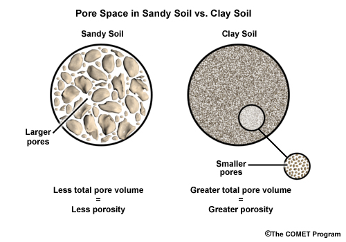
Fundamentally, it comes down to whether water moves to the stream over the land surface (as overland flow) or underground (as subsurface or groundwater flow). Even though a landscape might be covered with grass or trees, it’s still a lot easier for water to move downhill at the surface than to work its way through pores a few microns in size in soil and rock. Even when macropores are acting as super-highways of subsurface flow, they are still smaller, more tortuous, and less well connected than surface flow paths.
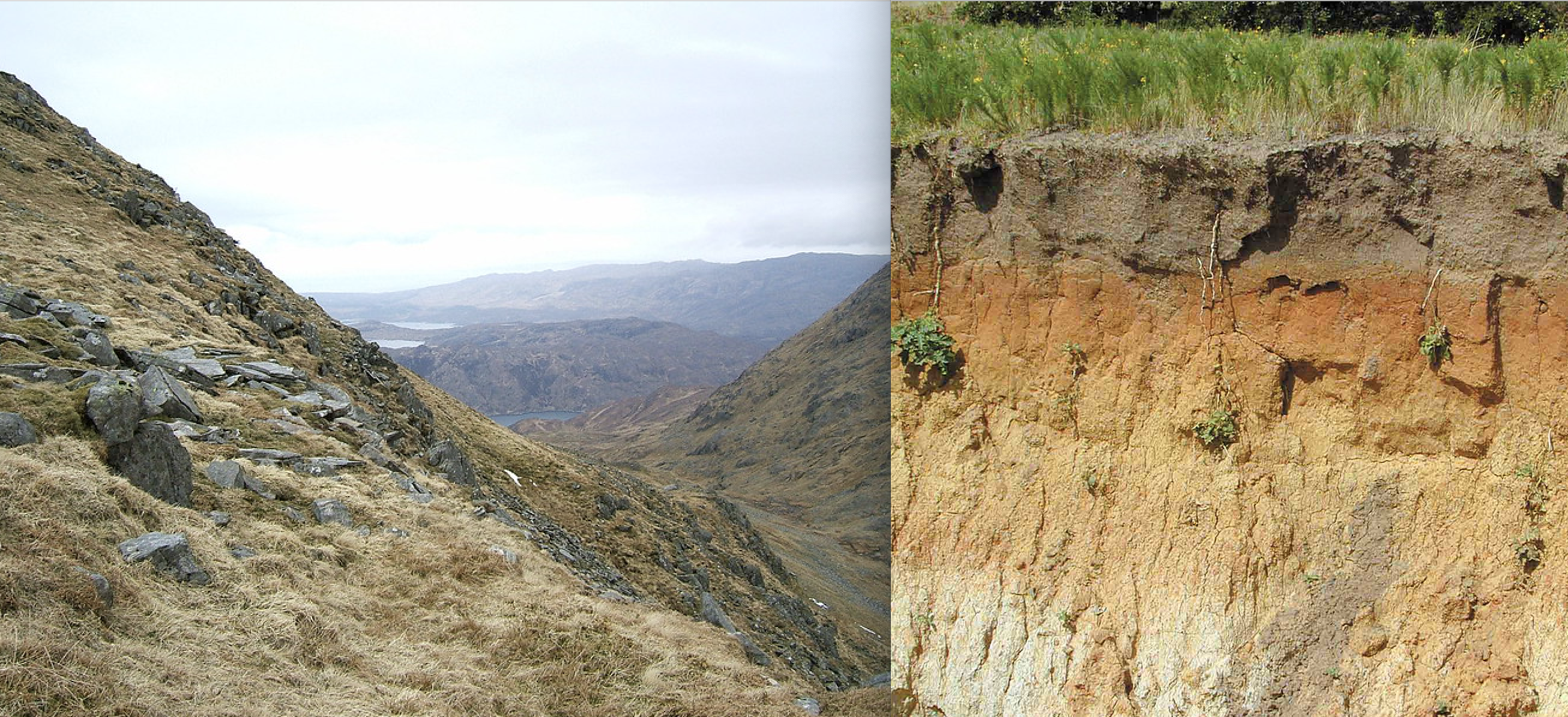
Imagine you are water. Which way easier to move downward – flowing overland on the rough slope or squeezing through tiny pores in the soil?
Photos by Lhoon on Flickr and the Noble Research Institute.
If you have a very small headwater stream that is fed by a few hillslopes, and water gets down those hillslopes very quickly, it doesn’t matter whether the rain drops fall on the top of the slopes or the bottoms, all of the water will arrive in the stream at very similar times. And if all of the water arrives in the stream at once, you will get a very high peak flow. But if your water movement is slower, then rain falling on the upper parts of the hillslopes will reach the a long time after the water from the rain that fell on the lower parts of the hillslopes. With those staggered arrivals, you will get a lower peak flow.
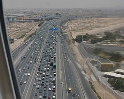
How are roads like streams? (Photo by Michael Coghlan from Adelaide, Australia / CC BY-SA)
(There are analogies that you can make with rush hour on city streets and freeways. Can you think of them?)
Putting it together, overland flow is faster than subsurface flow, and faster flow on/in the hillslopes leads to higher peak flows in the streams. (There’s a little wrinkle here in terms of the way we are talking about speeds, but we’ll get to that in a few paragraphs and this works for now.) Said another way, the shorter the lag time between precipitation and streamflow response, the higher the peak flow.
Now let’s add some nuance and think about the streamflow generation mechanisms one by one.
Infiltration excess overland flow
Infiltration excess (or Hortonian) overland flow is generated when it’s raining too hard for the soil to infiltrate into the subsurface. So the water always stays above ground. A little bit gets caught in the microtopography and ponds, but most of it runs off downslope. Water flowing at the surface will quickly collect from sheet flow into rills, which funnel water efficiently into streams. These rills will form in the steepest paths downhill and the flowing water will smooth out the land surface, decreasing friction and increasing the velocity of flow. [In urban areas, where impervious surfaces promote infiltration excess overland flow (which we call stormwater), gutters and storm sewers make super-smooth, super-speedy pathways for water to flow.] It take just minutes for overland flow to reach the stream. And when it stops raining, overland flow will finish draining to the stream quickly, usually completely stopping within hours. Infiltration excess overland flow is the proverbial hare in the foot race – fast as a flash for a little while, then stops moving.
Groundwater flow
In contrast, groundwater flow is ssssssllllooooooooowwww. Water infiltrates, percolates downward to the water table, and then moves down the hydraulic gradient as a function of hydraulic conductivity and hydraulic gradient (more-or-less slope of the water table) until it reaches the stream. Almost all of this movement happens through pore spaces that are a few microns to tens of microns in size. It can take months to years for groundwater to move from a hillslope into a stream.
That doesn’t mean that if it rains on April 10, that a groundwater-fed stream won’t start to rise in July. Instead, the new water molecules that recharge groundwater as a result of a storm help raise the water table and steepen the hydraulic gradient. That in turn causes water molecules that were already in the aquifer (old water) to flow a tiny bit faster toward the stream. So, if it rains April 10, a groundwater-fed stream may rise on April 11-13 (i.e., groundwater-fed streams respond on timescales of days). But that slow groundwater movement will also keep flow in the stream for weeks to months between storms. Groundwater flow is the proverbial hare – it just keeps plodding along. [Karst is an important exception to this generalization.]
An important aside: velocity vs. celerity
For water that moves through the subsurface, there is an important distinction between velocity (the variation of a water molecule’s position over time) and celerity (the speed at which a signal is propagated). Velocity controls the transit time (or age) of the water in the system and affects things like weathering and contaminant transport. Celerity controls the hydrograph shape – how quickly water rises and falls in the stream. The difference between velocity and celerity exists for overland flow as well, but since both timescales are so short, it’s less important for our purposes.
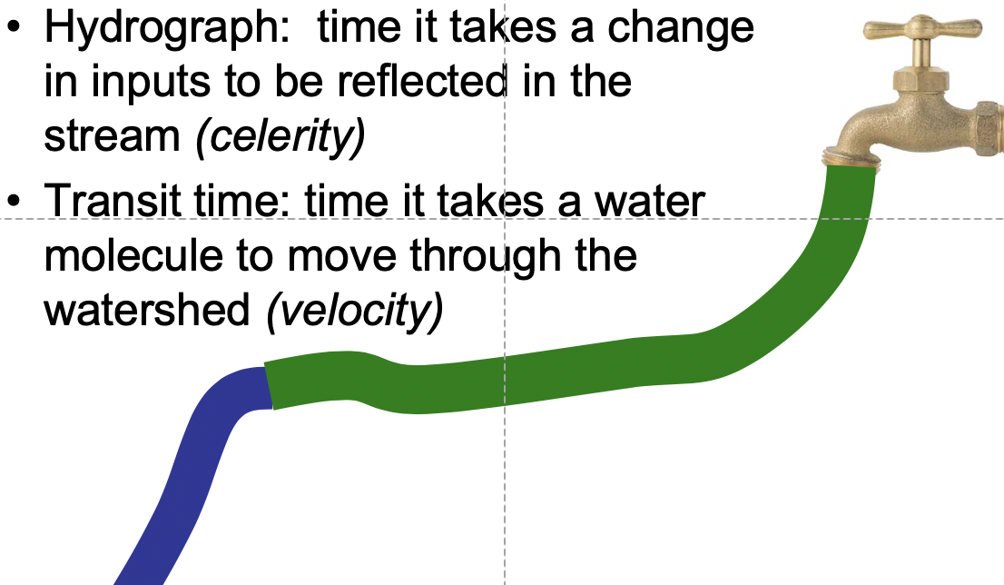
I like to think about water from the hose when I’m mentally separating velocity and celerity.
If you are struggling with the distinction between velocity and celerity, here’s the analogy I like to use: It’s a hot summer day, and you decide to get a drink from the hose. You turn the water on at the tap and water starts to come out the other end of the hose within a few seconds, so you bend down to take a drink. Ew!! The water is all hot and gross. But give it a minute or two and the water cools down and tastes much better. The quick response of water coming out of the hose as soon as you turn the tap on is a function of the celerity, but the change in temperature and taste is a function of velocity. Water coming from the tap pushes the old, hot water out the other end of the hose (celerity of the signal), but it takes a while for the fresh cold water from the tap to make it down the length of the hose (velocity of the molecules).
The illustration below may also help. It is from Hrachowitz et al., 2016 Transit times – the link between hydrology and water quality at the catchment scale, WIREs Water.
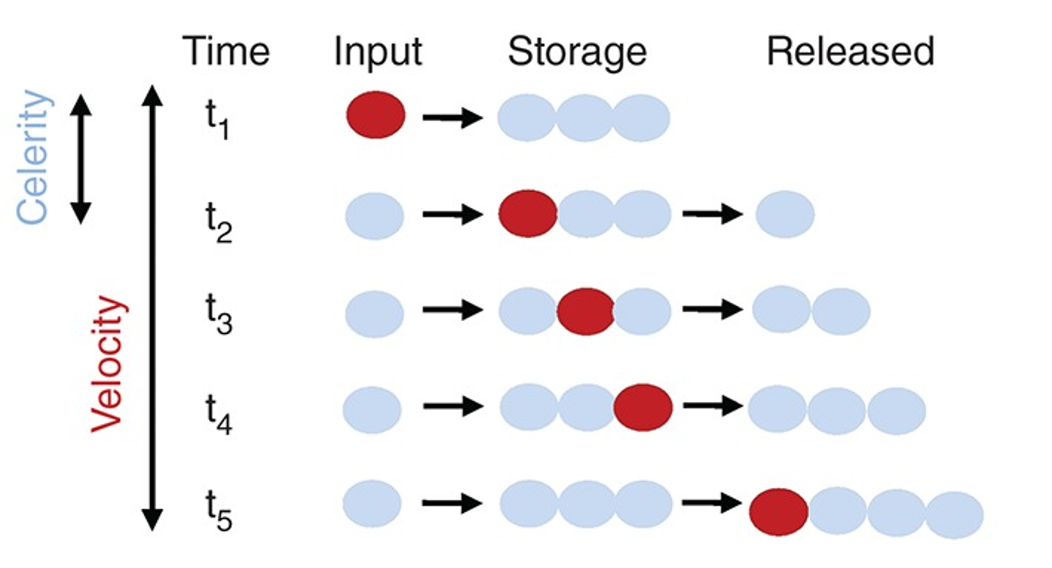
Follow what happens to the red dot over time vs. the release of water (i.e., cumulative streamflow) (Image from Hrachowitz et al., 2016, used under fair use)
So if infiltration-excess overland flow is the fastest and groundwater flow is the slowest, where do subsurface stormflow and saturation overland flow fit in?
Subsurface stormflow
Subsurface stormflow exploits macropores and preferential flowpaths to move through the subsurface more quickly than most groundwater flow. It also doesn’t go as deep in its path from hillslope to stream. But it’s still in the subsurface, so the velocity of the water molecules is still quite slow and transit times are likely in the range of weeks to months. However, preferential flow paths help accelerate the celerity of response. New water moving rapidly downward in preferential flow paths helps generate saturation just above the lower conductivity layer, increasing hydraulic conductivity in the soil and increasing the hydraulic gradient. That causes old water to move out of the soil and into the stream, raising water levels in the stream within a few hours of the rainfall.
Saturation Overland Flow
Now let’s get to saturation overland flow, which is the trickiest to wrap our heads around because it’s really a combination of all of the above. Where saturation overland flow is occurring, water is moving on the land surface and everything I said about infiltration excess overland flow applies. It’s fast and efficient. And for the direct precipitation on saturated areas, that’s all that matters, and timescales of response are in minutes.
BUT! Some of the water that becomes saturation overland flow is “return flow”, i.e., it is subsurface stormflow that has returned to the surface because the water table has reached or exceeded the surface elevation. So then we have to think about the relevant time scales for subsurface stormflow and for transit times, that means return flow overland flow may be weeks to months old. For hydrograph response (celerity), it may be hours, not minutes. Add direct precipitation and return flow together, and you end up with a hydrograph response from saturation overland flow that is a bit slower than you get with pure infiltration-excess overland flow.
Remember also that it takes time to saturate different pieces of the landscape – that’s related to the variable source area concept – so in whatever period exists between the start of rainfall and developing saturation overland flow in a particular area – everything I wrote about subsurface stormflow is what applies.
Real Watersheds
This is true more generally. No watershed has a completely spatially uniform response to a rainstorm. There is always going to be some mix of flow generation mechanisms happening, because of variability in soils, topography, vegetation and human impacts even in small areas. This means that no one scenario above is going to apply for a whole watershed – even during a single storm – instead it will be a blended, splendid mess that you will try to interpret in the context of the watershed characteristics and flow generation mechanisms that are likely to be at work.
As you get to larger watersheds, these flow generation mechanisms still matter and are likely to be even more heterogeneous, but the shape and size of the channel network also starts to matter a lot. At some point (~50-100 km2), the channel network tends to become much more important than the hillslopes. We’ll pick up on that theme in the coming weeks.
Where does this leave us? What’s the TL;DR version?
- There is a difference between velocity and celerity. Celerity is what matters when we are trying to connect flow generation mechanisms to hydrograph responses. But velocity matters for other things, like water quality.
- Infiltration excess overland flow generates the fastest hydrograph response (smallest lag time) – and the highest peak flows.
- Urbanization promotes infiltration excess overland flow, which is why urban streams are so notoriously flood prone.
- Saturation overland flow also results in fast hydrograph responses and high peak flows, but not quite as extreme as infiltration excess overland flow.
- Both overland flow mechanisms can give us peak flows that occur * Subsurface stormflow produces a hydrograph response within hours in small watersheds and it’s peak flows can be big, but not as big as those from overland flow.
- Groundwater is slow but steady and mostly supports baseflow. Left on its own, it produces peak flows that are much, much smaller than any of the other flow generation mechanisms.
- Real watersheds, even small ones, rarely have a single flow generation mechanism operating at all times. That means that real hydrograph responses are going to have a mixture of the characteristics described here and we can’t usually invert a hydrograph to tell us what flow generation mechanism produced it.
In graphical form:
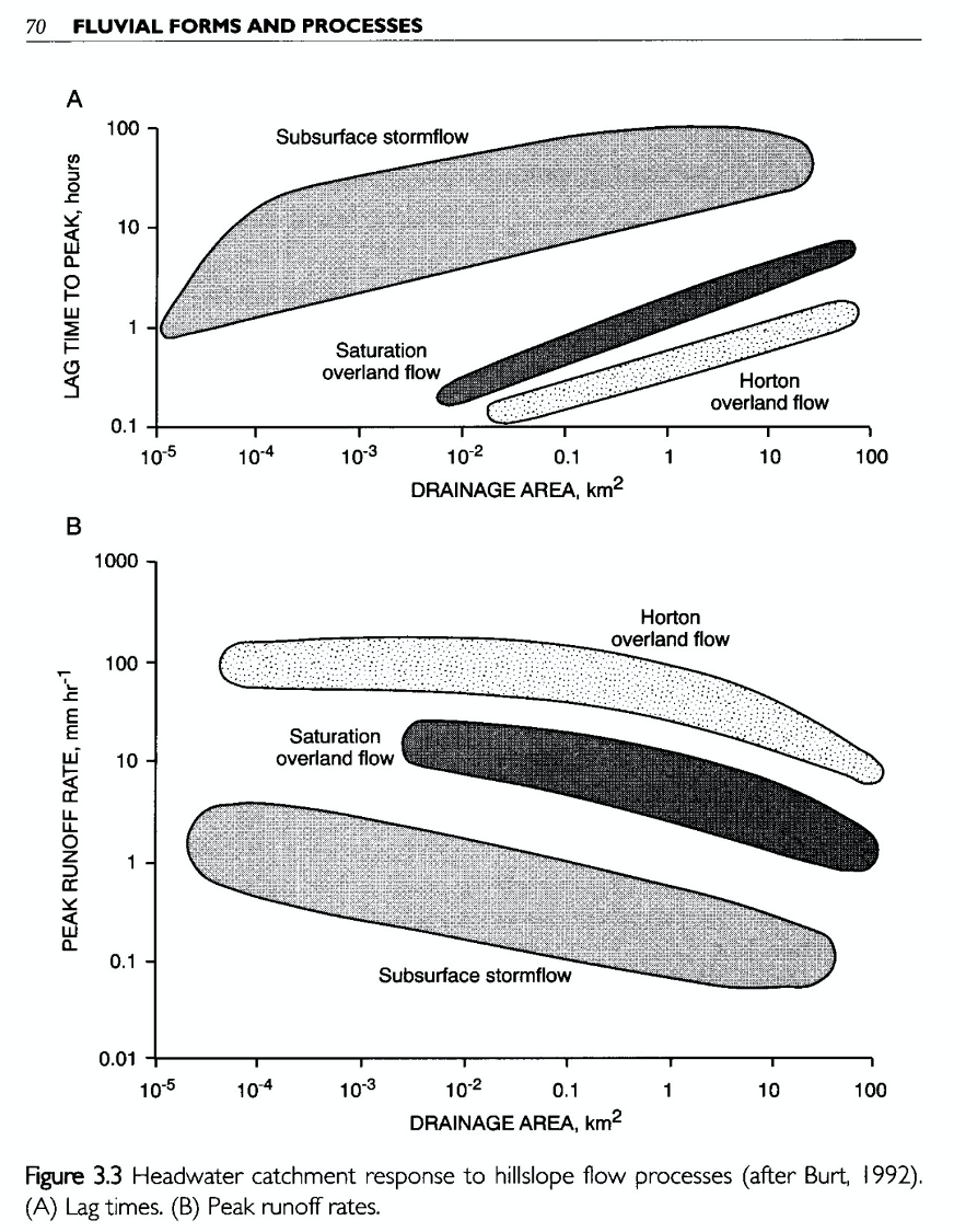 Does this figure make sense based on what you’ve read? It’s from David Knighton’s Fluvial Forms and Processes book (used under fair use).
.jpg)