![]() On March 9th, 1847, the world lost a great scientist to breast cancer. She was poor, lacked formal education, and practiced a minority religion, but she had a keen eye and mind that helped see things that others couldn’t and interpret them in new ways. Her discoveries made other men famous, but she was excluded from the scientific circles that discussed her findings. Despite this, she carried on making findings and describing them throughout her life, winning the respect of the gentleman scientists of her time.
On March 9th, 1847, the world lost a great scientist to breast cancer. She was poor, lacked formal education, and practiced a minority religion, but she had a keen eye and mind that helped see things that others couldn’t and interpret them in new ways. Her discoveries made other men famous, but she was excluded from the scientific circles that discussed her findings. Despite this, she carried on making findings and describing them throughout her life, winning the respect of the gentleman scientists of her time.
Maybe this is why the story of Mary Anning fascinates us still today, because it speaks to science and society and the ways that they sometimes uncomfortably interact. We like to presume that science is purely about the pursuit of truth and understanding the world around us. Yet who we allow to become scientists, to receive training and to earn recognition is dictated by societal constraints. And in turn these constraints may narrow the scope of scientific investigation, ultimately limiting the knowledge that is discovered and applied. And maybe we recognize that the same constraints that limited Mary Anning’s participation in the full practice of science are still at work today, just more subtly.
Or maybe it’s just that Mary Anning made her first major discovery at age 12, an age young enough that dinosaur- and fossil-obsessed six-year olds can picture themselves scrambling along cliffs or beach and finding a fossil that changes the way we think about life on earth, past and present.
I’ve written about Mary Anning and her town of Lyme Regis before, so in remembrance of her life and in honor of the contributions of all scientists kept from their full potential by the constraints of history, society, or fate, today I’ll just share a few more pictures of Anning, her fossils, and the landscape in which she worked.

A portrait and description of Anning in the fossil gallery of the Natural History Museum in London. Click for larger.

The first articulated plesiosaur discovered… by Anning on display in the Natural History Museum. The walls of this gallery are lined by fossil reptiles, many collected by Anning.

A landslip near Lyme Regis. The cliffs here are very unstable, and have small failures after every storm. This makes them a great spot for collecting fossils – and very dangerous.

Close up of the Blue Lias Formation at Lyme Regis. The alternating layers of limestone and shale laid down in a shallow Jurassic sea explain why this formation can be both a cliff forming outcrop and so incredibly unstable. Fortunately, the conditions were nearly perfect for fossil preservation.

The wonderful museum in Lyme Regis, built on the site of Anning’s house and first fossil shop. Today the museum is full of fossils and historical artifacts, mostly from Anning and her contemporaries.

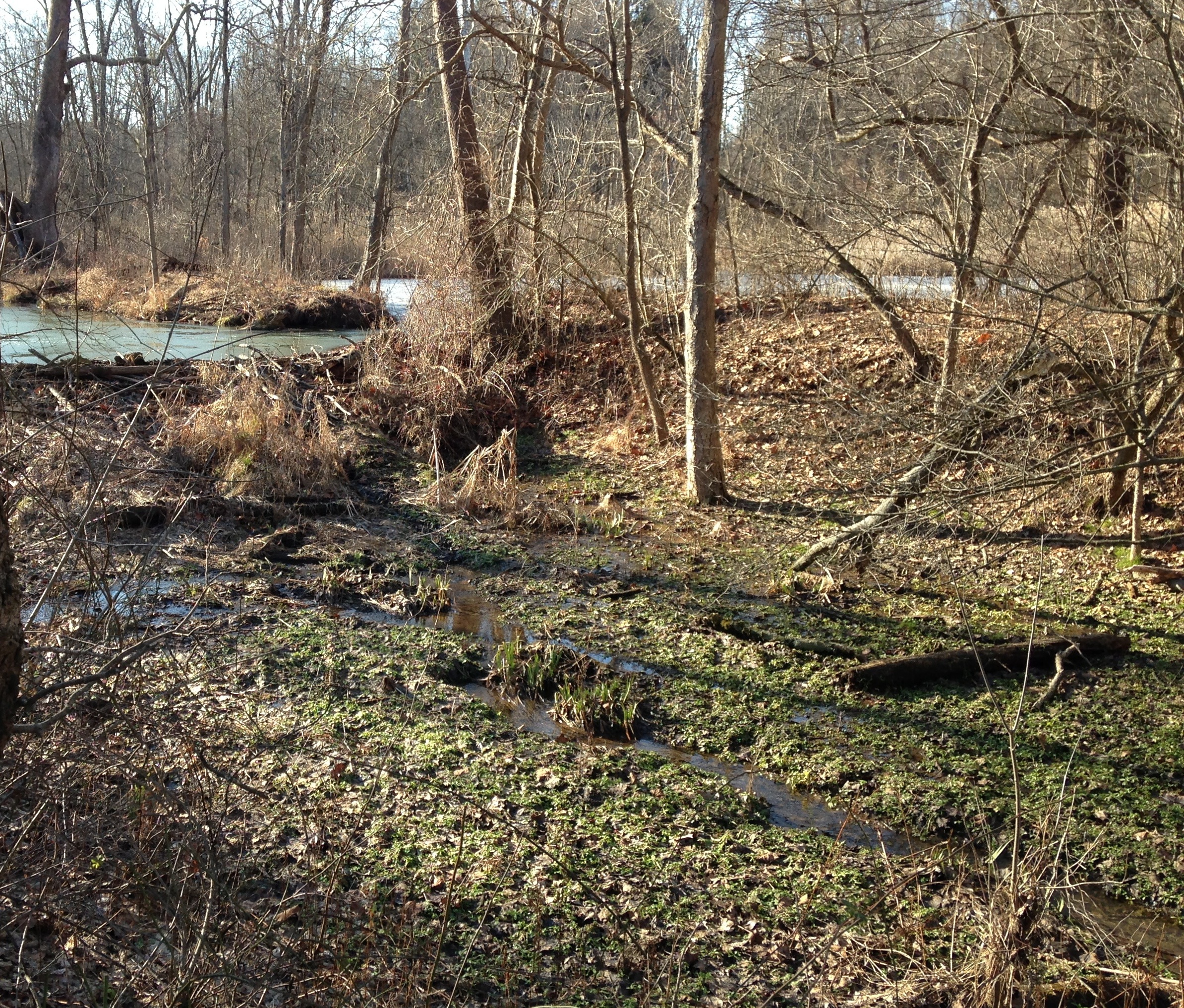
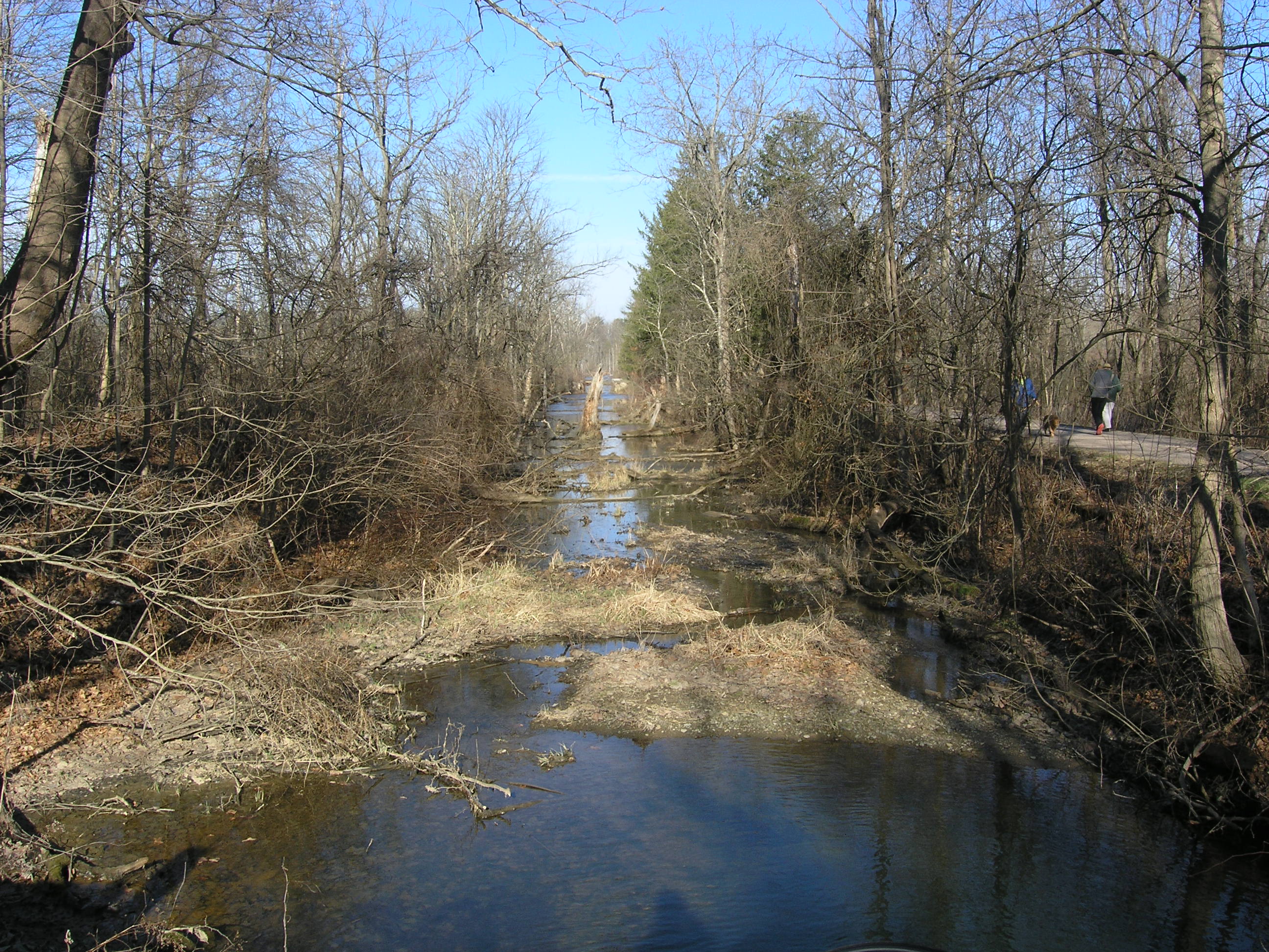
A little stream that flows to the sea through the heart of Lyme Regis. I like to imagine Anning crossing it on her way between home and outcrop. It may have looked quite similar to this during her time.