I thought that a useful follow-up to the musings on trust and access to scientific data prompted by the other week’s tale of near disaster would be to describe in detail how the measurements that I make in the lab are distilled into the results reported in a typical scientific paper, so you can see exactly how much information is included – and how much is left out. As an added bonus, you get to discover exactly what it is I do all day. It might be worth your while reading some background information before you continue.
The starting point for any palaeomagnetic study is a trip to collect drill cores. Having found a suitable sequence of lavas or sediments of the right age and location, we sample a number of sites at regular intervals through that sequence, collecting five or six cores from each site. We want duplicate samples from each site to check for consistency, and the sites spread across a large enough thickness of rocks to properly represent the long-term geomagnetic field direction, rather than a quirk of secular variation.
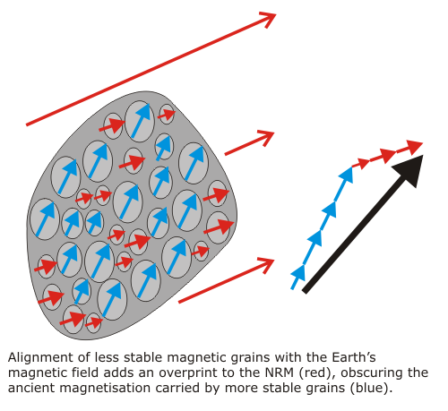
Back in the lab, we cut the cores down to a size that will fit in the magnetometer. Each individual core will generally yield between one and three samples, so by this stage we have a lot of chunks of rock to deal with; on my trip to KwaZulu-Natal, I drilled about 100 cores and ended up with around 160 samples. Unfortunately, extracting a useful palaeomagnetic direction from a sample is not a simple matter of placing it in the magnetometer and making a single measurement; the natural remanent magnetisation, or NRM, of an individual sample is made up of contributions from every magnetic particle it contains, and it is very unlikely that all of them are carrying the signal we’re looking for. As with every mineral in a rock, there will be a range of grain sizes, and therefore a range of different magnetic stabilities. Both very fine and very coarse grains are poor recorders of the ancient magnetic field, because they are too easily reset to a more modern field direction by random thermal fluctuations. Amongst the more useful, moderately sized particles (of the order of 100 nm, or 0.0001 mm, in diameter, which explains why we generally target mudstones rather than sandstones), later tectonic activity and igneous intrusions can reset even quite stable grains.
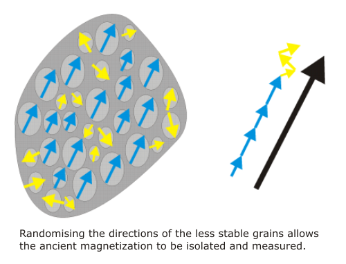
We hope that, buried beneath all the overprints, the most stable magnetic particles still carry a signal dating from the time of formation. To find out, we have to get rid of the less stable components, by shielding our samples from the Earth’s magnetic field, and then either heating them up or hitting them with an alternating magnetic field. This randomises the contribution of grains below a certain stability (because there is no ambient field for them to align with when they are reset), leaving a remanent magnetization produced only by the more stable grains. The higher the temperature or field, the more stable the grains that are randomised, and if we get this demagnetization exactly right, all of the overprints are removed, leaving only the original signal carried by the most stable magnetic grains.
Of course, we don’t generally know what the right temperature or field strength is, and we don’t want to overshoot and destroy the magnetisation we’re trying to isolate, so what we do is work upwards in tiny increments: you measure a sample’s magnetization, zap it with a slightly stronger field or temperature, then measure it again, then zap it again, and so on, until all of the NRM has been destroyed. At the end of this process, we might have measured the magnetization of each sample ten times or more. In the pseudo-3D plot of a typical demagnetisation sequence below, the endpoints of the measured remanence vectors sweep out a path in three-dimensional space as the sample’s NRM is progressively removed, with the difference between consecutive remanence vectors indicating the orientation of the component presently being randomised.
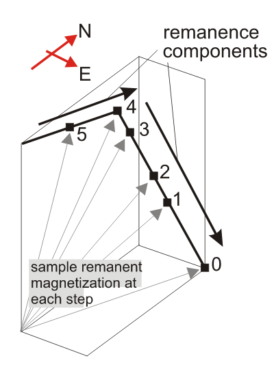
In this example, the first four endpoints are moving upwards in an approximately easterly direction, signifying the removal of an east- and downwards pointing remanence component. After point 4, however, the demagnetisation path changes direction, revealing a flat, northeast pointing remanence hidden beneath initial overprint. This more stable component decays towards to origin, indicating that it is being carried by the most stable magnetic grains in the sample (if there was a third component yet to be uncovered, the demagnetisation path would be missing the origin), and is therefore the most likely to record a magnetization acquired at the time the rock formed. Having rotated the data into the correct spatial reference frame (which I’ve explained before) we can calculate a best-fit direction for these points, which gives us one measurement of the ancient magnetic field. Do this for every sample, and plot them on a stereonet, and you should get something like this:
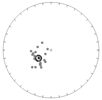
The inherent variability of the geomagnetic field, plus the cumulative errors in core orientation and measurement, mean that we expect the scatter of individual points about the calculated mean direction (the black square). We usually also calculate a 95% confidence interval (the black ellipse) – the “real” mean direction represented by these data has a 95% chance of falling within this interval. The mean direction is the jumping-off point for any larger-scale analysis of, for example, the past motions of tectonic plates, so from a certain perspective, all that laboratory grunt work – multiple measurements of dozens of samples – has gone into producing just three relevant numbers for each site you sample: the bearing and inclination of the mean direction, and the confidence interval associated with it. It was for this reason that some of my friends once joked that I should walk into my PhD viva with nothing but a giant arrow as a prop.
It does, however, present a problem when you’re writing up: you want to spend as much time as possible in a paper analysing what your palaeomagnetic results mean – which is generally where the novel science lies – so you don’t want to use more pages than necessary presenting the reams of raw data behind each of your mean directions. For this reason, even in a well-documented study the information you get is somewhat limited:
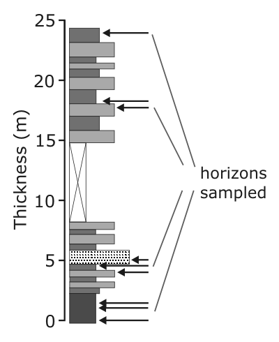
- The location and a brief description of the studied sequence, sometimes with a stratigraphic log indicating horizons which were sampled.
- A description of the demagnetisation procedures used: the techniques, and the intensity of the applied steps.
- Demagnetisation behaviour described in general terms, with a number of representative demagnetisation plots (following corrections for core orientation and bedding tilt) for illustration.
- A stereonet plotting best-fit directions for each sample and the site mean.
What is presented allows the reader to confirm that sampling has been performed appropriately, that at least a few of the samples exhibit decent demagnetisation behaviour, and that the individual directions contributing to your site mean are not scattered all over the stereonet. As I’ve discussed before, this is a confirmation in principle that you’ve followed the right procedures, and that your data superficially say what you claim. But there’s clearly a lot missing: for example, with demagnetisation data for only a handful of samples, when dozens were analysed, no-one can confirm for sure that your ‘representative’ plots really are representative, and that the line fits displayed on the stereoplots are appropriate. Does this matter? Given that this post is already over-long, I’ll save my thoughts on that for later – but if anyone has made it this far, I’d be interested in your views.
Addendum: For anyone who wants to get really into the technicalities, here are a few of good online resources:
- Paleomagnetism: Magnetic Domains to Geologic Terranes – online version of an excellent (but out of print) introductory text.
- Lectures in Paleomagnetism by Lisa Tauxe.
- The Hitchhiker’s Guide to Magnetism

Comments (6)