Measuring evapotranspiration components

Evapotranspiration is often said to be the most difficult water balance component to directly measure. When water goes from liquid to vapor, you can’t exactly catch it in a bucket or measure flow in a channel. In my Watershed Hydrology class, we used a very simplified version of the weighing lysimeter to measure evapotranspiration from soils and potted plants. But how else can we measure evaporation and transpiration? Let’s start by talking about techniques used to measure evapotranspiration from particular surfaces (open water, soil, plant interiors (transpiration), and plant surfaces (interception)).

1. Open Water Evaporation

As we talked about in class, open water evaporation is first and foremost a function of the availability of energy (i.e., net radiation) at the water surface and the ease with which water vapor can mix into the atmosphere (i.e., humidity, wind). But properties of the water body also matter, including water depth, thermal stratification, size, heat content of inflows and outflows, vegetation (shading), turbidity and bottom reflectance (albedo), and salinity. Unfortunately, those variable water body properties make it a harder to get evaporation than it would be if it were solely energy, wind, and humidity.

If you want to measure lake evaporation, one approach is to measure all of the other hydrologic cycle components for the lake, including change in lake level for your change in storage. Then solve for evaporation, using the water balance. 

lake with arrows showing precipitation, evaporation, and surface and groundwater inflow and outflow

Example of the components needed for a lake water balance. This image is from the USGS, http://pubs.usgs.gov/wri/wrir-03-4238/ and is in the public domain.

If the water balance approach is not practical, you can measure the water balance of a very simplified system called an evaporation pan. Here’s how a standard (class A) evaporation pan works. The pan is 122 cm in diameter and 25 cm deep. It’s placed outside in an area free of obstructions and water level is maintained at 18-20 cm deep. The water is refilled as needed to maintain the desired level. Water level measurements are taken daily (giving evaporation as a depth) or the volume of water required to refill to the desired level is recorded (volume of added water divided by area of pan = evaporation as depth). Of course, since the pan is outside, it will also receive rainfall, so that needs to be measured and figured into the calculations:

Evaporation = beginning depth – ending depth (for days with no rain)

Evaporation = beginning depth – ending depth – rainfall depth (for days with rain)

Since a shallow pan evaporates more quickly than a deeper lake, to get lake evaporation you  multiply the pan evaporation rate from the pan by a lake coefficient (typically 0.7 to 0.75) that takes that into account.

Metal pan filed with water with a fence over the top, on a pallet in a mowed area.

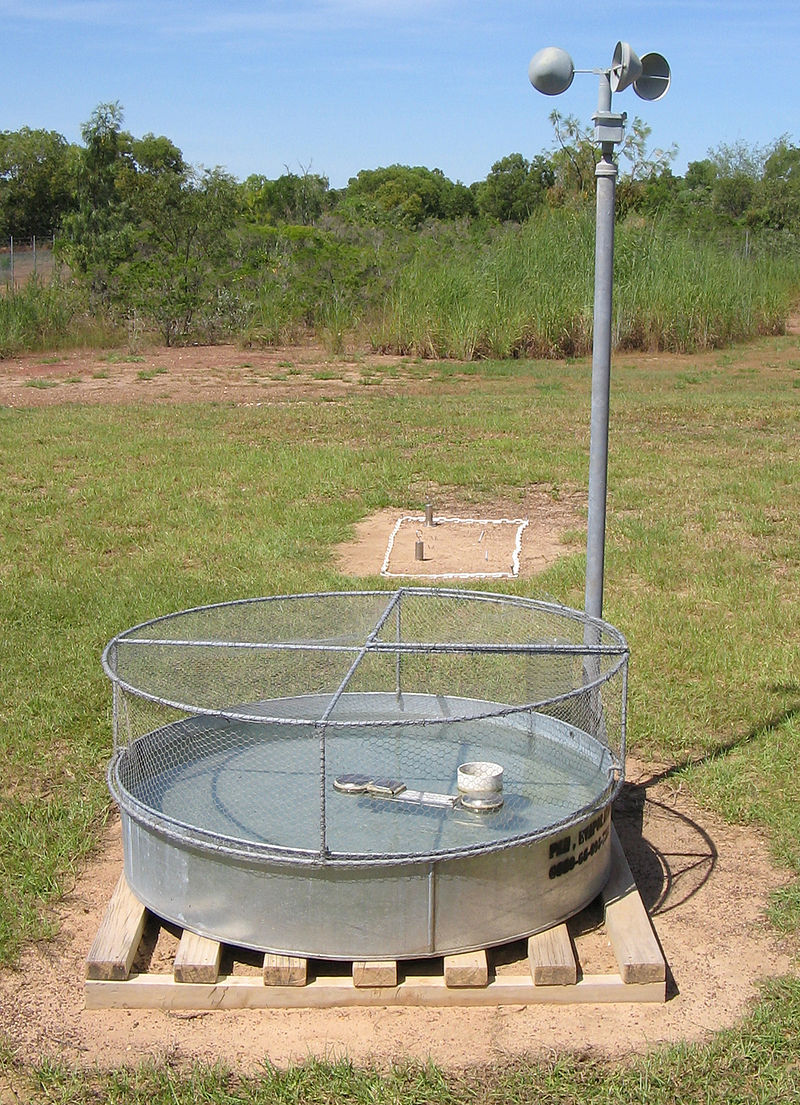
A Bureau of Meteorology (Australia) class A evaporation pan, with an adjacent anemometer to measure wind speed. A rain gauge would also be located nearby. This file is licensed under the Creative Commons Attribution 3.0 Unported license from Wikimeida. Image by Bidgee.

2. Soil evaporation

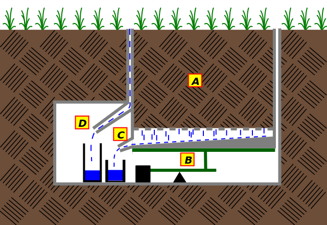
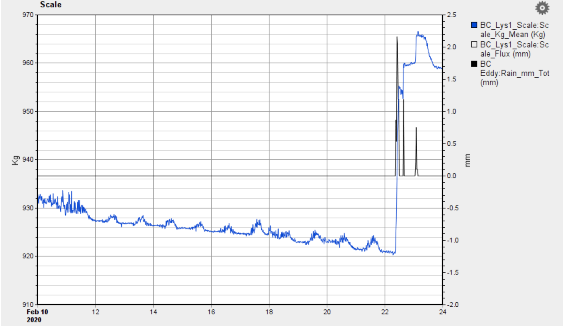
The conceptually simplest way to measure soil evaporation is the weighing lysimeter, as long as your lysimeter doesn’t contain any vegetation. (The group who used the pots with soil and mulch was measuring soil evaporation in this approach.) The weighing lysimeter takes advantage of a mass balance approach to the water balance.

Another method takes advance of a heat balance. In this technique, fine scale measurements of soil temperature and thermal properties are used to calculate change in sensible heat storage at different depths from the soil surface. Over short distances and time scales, sensible heat changes as a function of latent heat (i.e., evaporation).

Measurements are made with carefully spaced thermocouples (i.e., thermometers). One of the thermocouples also has a heating element, that can send out pulses of heat. By measuring how those heat pulses are received at different distances, the latent heat can be calculated.

three pronged sensor with 3 thermocouples and a central heater. Variables are named in relevant positions.

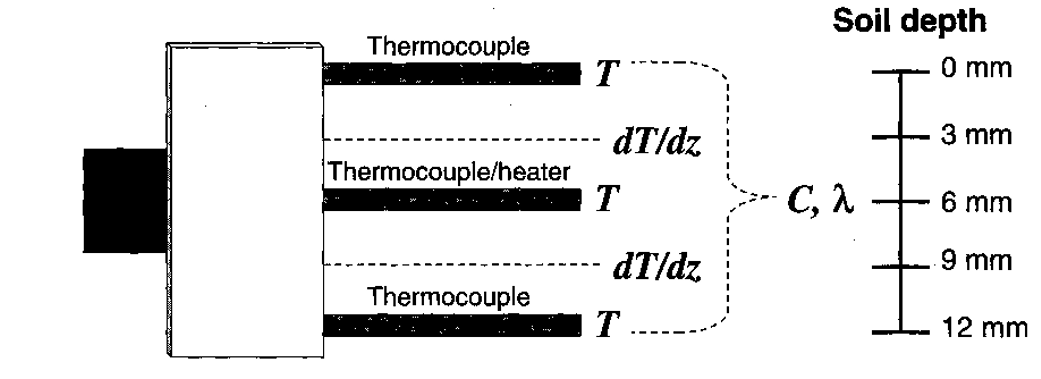
Heat pulse sensor and associated measurements. Temperature (T), temperature gradient (dT/dz), volumetric heat capacity (C), and thermal conductivity (I) are the relevant variables. From Heitman et al., 2008, Water Resources Research.

You can read a lot more about the details of the method and math in Heitman et al., 2008, Water Resources Research, which is freely available. The diagram above shows how the apparatus works. Looking ahead, this approach is very similar to how sapflow in trees is measured to estimate transpiration.

3. Transpiration (evaporation from plant interiors)

Transpiration – or evaporation from the leaves and needles of vegetation – is really important in many landscapes. You’ve already experienced one approach to measuring it – our variation on the weighing lysimeter – with our potted plant experiments.

Measuring the change in weight of potted plants is a tried-and-true approach to estimating transpiration – especially if care is taken to reduce soil evaporation (think mulch or some sort of plastic sheeting). But there are limits on how big a plant you can put on a scale and larger weighing lysimeters can be very expensive to build and maintain. Even then, you don’t find many weighing lysimeters measuring full grown oak or fir trees! So other approaches are needed.

An approach that works with plants up to large shrubs or small trees is the tent method. Here the plant is enclosed in a clear plastic tent and the moisture content of the air entering and leaving the tent (via fans) is measured. When the moisture content of the air leaving the tent is higher than the air entering the tent, that’s because of evapotranspiration. And if the soil surface is covered, the difference in moisture is just due to transpiration.  BUT! It gets hot inside the tent so maintaining proper air flow is critical. Even so, the transpiration rates measured using the tent method might not be the same as would occur in the surrounding natural environment.

line drawing of leafy plant inside clear plastic tent with some sort of single level inlet and multi-level outlet structure

Illustration of the tent method for measuring evapotranspiration. Figure 4.5 in Brooks et al., 2012, Hydrology and the Management of Watersheds (your textbook).

A smaller, shorter-term variation on the tent method is porometry – which measures stomatal conductance. In porometry, a leaf is temporarily enclosed in a small chamber where changes in humidity are measured – and attributed to transpiration. Porometry is good at telling scientists how stomata are responding to environmental variations at really small scales, but isn’t good at providing larger scale data, because what the stomata are doing  can vary depending on the orientation of the leaves,  height in the tree, etc. Age of the plant, plant species, etc. also effect how stomata respond to environmental conditions – and that’s before you even get to the environmental variations themselves (temperature, humidity, wind, etc.). So you would need to make a LOT of stomatal conductance measurements via porometry to use this approach to accurately measure transpiration for large plants, like trees, for example. Nonetheless, it’s a pretty cool technique that can tell you a lot about how plants are taking up and releasing water. Here’s a video that explains more about how it works:

So if porometry, tenting, and weighing lysimeter style measurements are all limited to small plants, how the heck do you measure transpiration in larger trees? After all, in forested environments, they are going to be doing a lot of the transpiration we’re interested in. The answer is sap flow measurement, and here are two videos that explain what it is and how it works. The first video gives you a quick and simple explanation, while the second video is full of information and even shows example data!

4. Interception (evaporation from plant surfaces)

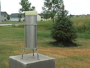
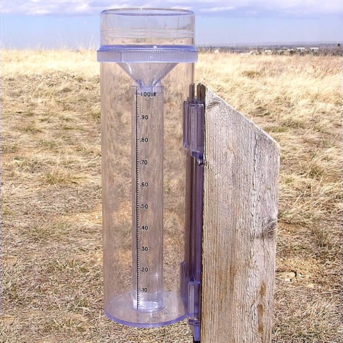
Interception is the precipitation that never makes it to the soil surface because it gets hung up on leaves and branches of vegetation or even the dead organic material on the forest floor (the litter). After the storm is over, this water evaporates before it ever reaches the ground. That process of being caught then evaporated is called interception. Interception can be a very important water balance term, in both the winter and summer. (I’ve written more about snowfall interception here.)

The simplest way to measure interception is to measure the precipitation in an open area and compare to precipitation measured under the forest canopy (through fall) and what runs down the stems of trees (stemflow). Interception is the difference. This ignores litter interception though and that’s a bit harder to measure. There are also some really cool new techniques demonstrated in the video below, that let researchers start to scale up from point measurements to a whole forest:

Categories: by Anne, hydrology, teaching

Measuring actual evapotranspiration with weighing lysimeters

In my Watershed Hydrology class this semester, we conducted student-designed experiments with potted plants and bare soils to study the factors affecting evapotranspiration. The procedure we used is a simplified version of a weighing lysimeter.

How a lysimeter works

Weighing lysimeters are one of the very best ways of measuring the actual evapotranspiration from a small area of land, because they use mass balance (i.e., changing weight) to give us the combined total of plant transpiration, soil evaporation, and interception losses over time. Our class potted plant experiments were in the laboratory, but in order to understand the effects of environmental variability on evapotranspiration rates, most weighing lysimters are installed in the outdoors – what we called “in the field.”

land surface, soil, and underground laboratory showing water being collected
Weighing lysimeter schematic. A is the soil monolith, B is the load cell (weighing mechanism), C is the deep drainage being collected, and D is a measurement of surface runoff being collected. The illustration was created by Giancarlo Dessì and is used under a CC BY-SA 2.5 license, via Wikimedia.

Here’s how a weighing lysimeter works: A large soil core (called a “monolith”) is carefully removed from the ground and put inside a cylinder or box (A in the image above). The monolith-in-a-cylinder is then placed back into the ground and vegetation is planted. The cylinder usually will have a drain in the bottom so that water that percolates downward through the soil can leave the cylinder and be accounted for as a deep drainage loss (C in the image above). The cylinder sits on a load cell, which is like a giant scale that continuously records the weight of the soil (B in the image above). Decreases in weight are associated with evapotranspiration and deep drainage, but since deep drainage is often measured separately, it can be split off and the mass lost because of evapotranspiration can be accurately measured. Some weighing lysimeters may also have a way of accounting for surface runoff generated in the cell as shown in D in the image above, some will have sensors embedded in the soil measuring moisture content and other soil properties, and most lysimeters will have a nearby weather station including a rain gauge.

Lysimeter math

Weighing lysimeters take advantage of the water balance equation:

Input – Output = Change in Storage

The construction of the lysimeters simplifies the inputs and outputs, by removing complications like lateral groundwater flow.  The equation becomes:

Precipitation – Evapotranspiration – Deep Drainage = Change in Storage

[Sometimes surface runoff will also be included, as shown in the figure at the top of the post. However, this is avoided where possible.]  Rearrange the equation and solve for evapotranspiration:

Evapotranspiration = Precipitation – Deep Drainage – Change in Storage

Precipitation and deep drainage are measured directly, with a rain gauge and the collection device shown in the image. The changing weight of the lysimeter measures the change in storage of water in the soil and plants. Taken together, that means the only unmeasured term is evapotranspiration, so the numbers can be put into the equation and voila…evapotranspiration.

And because most lysimeters constructed these days have digital load cells and data loggers, they collect high frequency data. This means we can calculate evapotranspiration at the time scale of minutes, hours, days, … or whatever timescale is of interest.

Lysimeter data

Let’s look at some data from a real lysimeter. This lysimeter is operated by the Desert Research Institute in Nevada. This lysimeter is one of three lysimeters, each 2.2 m diameter and 3.0 m depth filled with soil from the Mojave Desert. In the graph below, you can see the mass decrease during each day as evapotranspiration removes water (and mass) from the system. At night, there is a very slight increase in mass coinciding with dew or frost formation on the soil. This is a telltale sign that mass decrease is evapotranspiration and not drainage – we wouldn’t expect drainage to stop at night or have a fairly constant rate day after day.

Graph showing decreasing mass over time then abrupt increase in mass with rainfall.
DRI lysimeter data from the last two weeks. Decreases in weight show evapotranspiration fluxes. What happened when it rained?

On February 22nd, the site got some rain, and you can see a near instantaneous increase in the mass of the soil. After the rain ends on about February 23, you see a rapid decline in mass up until the end of the graph. This rapid decline may represent a period when there is deep drainage of water from the soil monolith. Note how much faster it is compared to the evapotranspiration losses earlier in the graph.

You can read more about the Nevada lysimeters here and look at all of the great real-time data they post to the web.

Look at some real lysimeters

As you can see, a real-life weighing lysimeter is quite a bit more sophisticated than the periodic measurements of the weight of a potted plant that we’ll be doing in class this week. But the concept is the same, and weighing lysimeters come in a range of sizes. You can read more about how two large lysimeters helped California scientists learn more about orchard and vine crop water use here. The California link has some great photos the lysimeter construction, old-school measurement techniques, and the sort of analyses that can be done with the data.

The videos below show the installation of a small weighing lysimeter and the construction of a series of rather larger ones. (The second video is in French but has English captions.)

This video (in German) shows the underground laboratory where the lysimeter data and water samples are collected.

Obviously, large lysimeters are expensive to construct and are used for a lot more than just measuring evapotranspiration. Two of the videos above show how lysimeters can be used to gain insight into water quality problems. Also, sometimes it’s not necessary – or practical – to preserve an intact soil core or monolith. However, disturbed or constructed soils won’t have the same soil pore structure or other characteristics of natural soils – at least until they’ve had a chance to evolve for a few years. But regardless of the additional data collected or the way they are constructed, weighing lysimeters are unparalleled in their capability of fully closing the water balance and getting accurate measurements of actual evapotranspiration.

Categories: by Anne, hydrology, teaching

Measuring precipitation: radar and satellite based measurements

In the previous post, I reviewed approaches for point measurements of precipitation (i.e., rain gauges), talked about the care that must be taken to site well and minimize undercatch, and identified some of the common data sources for rain gauge measurements in the United States. Rain gauges do a great job of telling us how much precipitation is reaching the ground surface at the place where they are located, but the vexing problem is figuring out how well that point measurement represents a broader area of interest. So in this post, I want to focus on technologies that look to the sky to provide data on the intensity of precipitation occurring over broader areas.

Radar Rainfall Measurement

How does it work?

Radar systems have antennae that send out pulses of electromagnetic energy that are reflected off a targets and returned to the antenna. The energy return is used to calculate reflectivity (Z). Here’s a nice short (2-3 minute) explanatory video from the UK Met Office.

So the radar systems are measuring reflectivity from the rain, but how is that converted to rain rate? The reflectivity (Z) depends on the number of rain drops and their diameter. An increase in drop diameter increases reflectivity to the sixth power. So if rain drop diameter doubles, reflectivity increases by 2^6 = 64. This is important for calculating rate (R), because rate depends on drop diameter, the number of drops, and the drop fall speed. And bigger drops generate faster rainfall rates. An increase drop diameter increases rate to the 3rd power So if diameter doubles, the rate increases by 2^3 or factor of 8. The relationship between Z and R varies depending on atmospheric conditions, so there isn’t just one equation to apply. Z-R relationships are better understood for rain than snow (this is related to the snow depth versus snow water equivalent (SWE problem). Both hail and wet snow have high reflectivity relative to the Z-R relationship for rain. Z-R relationships are checked against and corrected using point rain gauge measurements. This increases their accuracy relative to a radar-only approach.

Once you’ve got an appropriate Z-R relationship, then rainfall amount is simply the rain rate times the duration. Since radar scans occur every few minutes, radar rainfall measurements can not only give total precipitation from a storm but also provide data on how intensity varies within it.

Where does the data come from (in the US)?

There is a network of 158 Doppler radar systems that cover most of the continental US, and this system is called NEXRAD. Doppler radar provides additional information on the motion of air using the Doppler effect in addition to the echosounding of traditional radar. These Doppler radar systems have a range of 230 km (125 mi) radius from where they are installed, so the network is designed to cover most populated areas. Data quality are best closer to the radar sites than at the fringes of the range, and mountainous topography can create data gaps. Within a few miles of the radar sites there can also be issues with data quality.

This slightly longer (8 minute) video explains how NEXRAD works and the many ways that the data are used.

NEXRAD was developed in the 1980s and deployed nationwide in the 1990s, so the instruments are aging and prone to breakage. The National Weather Service (NWS) is undertaking upgrades and planned maintenance to extend the life of the installations to at least 2030.

NEXRAD data are used for flash flood warnings and they are often incorporated into river flow forecast models. Beyond NEXRAD there are also smaller and even mobile radar installations that are used for more localized applications, including research and new technology development. Unless you are involved in a project using these installations, data may not exist, be available, or be appropriate processed for Z-R, for your area and the time you need it, so the the NEXRAD precipitation data are the go-to radar data for most hydrologic applications.

Where do I get access to the data?

Map shows intense rain in Sierra Nevadars and lighter rain over much of western US and Great Lakes region.

Screenshot of https://water.weather.gov/precip/ on February 6th, 2019, showing one day observed precipitation.

You can view one-day observed precipitation for the United States at https://water.weather.gov/precip/. That site allows you to zoom in to a particular area and select different dates from the archives. If you don’t want daily precipitation, you can add it up over longer periods. In addition to viewing data, you can download the data in several formats. Be aware that this is spatial data, so it’s not just a time series of measurements for one spot.

It's raining to our west and north.

Screenshot of the Cleveland NEXRAD image on the morning of February 6, 2019.

If you want to look at the NEXRAD data for the Cleveland site (which covers Kent), you can go to: https://radar.weather.gov/radar.php?rid=cle&product=N0R&overlay=11101111&loop=no. The default display is base reflectivity (Z), but if you look along the left column, you’ll see options for one hour and storm total precipitation. In the upper left corner, you’ll see arrows that let you move to adjacent NEXRAD sites and at the bottom you can click to view a larger region of the country.

In the US, daily radar precipitation measurements are publicly released for 4 km by 4 km grid cells (as shown at https://water.weather.gov/precip/), and researchers can access higher spatial and temporal resolution data from the National Centers for Environmental Information (also called the NCDC), including 1-hour precipitation, 3 hour precipitation, and storm total precipitation. Different spatial resolutions are available depending on whether the radar system scans the sky with a horizontal beam only or if it has dual polarization, which means that it scans with both horizontal and vertical beams.

Satellite Precipitation Measurements

This NASA video gives a great overview of the Global Precipitation Measurement Mission, which is an international mission to provide precipitation data for the Earth from 60 degrees N to 60 degrees S.

GPM logo - shape of a raindrop

Notice that the GPM logo is in the shape of a raindrop?

The Core Satellite has 2 instruments:

  • GPM Microwave Imager (GMI) (amount, size, intensity and type of precipitation)
  • Dual-frequency Precipitation Radar (DPR) (3D profiles and intensities of liquid and solid precipitation)

The satellite orbits 407 km (253 miles) above the Earth, with an orbital duration of 93 minutes. That means that it makes about 16 orbits per day. Thus, the data isn’t as a frequent as with ground-based radar, and its generally released . NASA offers the data at multiple levels of processing, but the highest quality rainfall data product is released at 0.1 degree (lat/long) spatial resolution. For our latitude, that’s a grid cell of about 11 km by 11 km, so it’s also coarser resolution than ground-based radar. What’s the advantage of satellite precipitation? Near global coverage. That means the data are available over the oceans and other places where ground-based measurements are sparse. For watershed hydrologists working in the United States, NEXRAD and rain gauges are more commonly used data sources, but if you are interested in working in other parts of the world or on really large scale hydro-meteorological phenomena, satellite products may be an invaluable resource.

Please note: The information above is designed for students in Kent State’s Watershed Hydrology class who are learning the basics of precipitation measurement. If you are an expert at anything in this post and discover an error, you can let me know with constructive pointers to better information.)

Categories: by Anne, hydrology, teaching

Measuring precipitation: rain gauges and point precipitation data sources

As watershed hydrologists, we care a lot about precipitation, especially when it reaches the land surface (or the vegetation just above it). Precipitation is the dominant input to our water balances and a major driver of streamflow and water table responses. Because precipitation is so important, we need to spend some time talking about how we measure it. Some hydrologists spend large chunks of their careers working out the best ways to measure and analyze precipitation (and understanding the processes that make it so hard to do!), so this is just an overview.

All about rain gauges

The simplest way to measure precipitation is to put a rain gauge at a point on the landscape. Almost all rain gauges have a funnel down to an opening that then drops water into a collection container. The amount of water in the container is either measured at specified intervals, or it is automatically measured and recorded. Knowing the size of the top of the funnel relative to the size of the collection container lets us related the volume or depth of water in the container to the amount of rainfall.

Standard rain gauges

Here’s what’s called a standard rain gauge:

Standard rain gauge, as pictured by the National Weather Service.

Standard rain gauge, as pictured by the National Weather Service.

This is what the Cooperative Observers for the National Weather Service (NWS) use to measure rainfall. Here’s how the National Weather Service describes the gauge: “The most common is the non-recording gauge called a Standard Rain Gauge, SRG. Typically the SRG is a metal cylinder with a funnel on top and a plastic measuring tube in the middle. The measuring tube can handle up to 2.00 inches of rain before overflowing into the larger outer cylinder. During the winter, the observer removes the funnel and inner tube and allows the snow to collect in the outer tube. The observer then melts the snow and measures it, getting an accurate water equivalent to report.” Dr. Jefferson has a standard rain gauge sitting in her office. Ask her to show it to you some time.

From that picture, you can’t see what the inside of the rain gauge looks like, but there’s a smaller version of it that a lot of people (include Dr. Jefferson) use. It’s the official rain gauge of the CoCoRAHS network (more on them in a minute).

4" rain gauge made by Stratus and recommended by CoCoRAHS. When more than 1" of rainfall is collected, it overflows from the inner cylinder to the outer cylinder. Then if you need to measure it, you can carefully pour increments of water into the inner cylinder and add it up. In the winter, you take off the funnel and inner cylinder and can collect snow,

4″ rain gauge made by Stratus and required by CoCoRAHS. When more than 1″ of rainfall is collected, it overflows from the inner cylinder to the outer cylinder. Then if you need to measure it, you can carefully pour increments of water into the inner cylinder and add it up. In the winter, you take off the funnel and inner cylinder and can collect snow.

The limitation of these rain gauges is that someone has to go outside and manually measure the water level in the gauge, so it is difficult to get frequent (sub-daily) measurements of rainfall. Enter the recording rain gauges.

Recording rain gauges

The National Weather Service (NWS) uses a recording rain gauge that weighs the collected precipitation every 15 minutes, converts that weight into a depth (again using the geometry of the funnel), and records the depth on a punch tape. Once a month, someone can visit the gauge, dump it out and put in a new punch tape. It’s old school, but it works accurately and with minimal maintenance.

Fancier still is the tipping bucket rain gauge. You should watch the video below to see how a tipping bucket rain gauge works. (The one in the video is heated to melt snow and ice, but not all tipping bucket rain gauges are.)

Tipping bucket rain gauges are appreciated for their ability to give high frequency data, because the data logger actually records every time the bucket tips (every 1 mm or 0.01 inch of rain). You can turn that record of tips into things like 5 minute rainfall intensity, which is fantastic. However, tipping bucket rain gauges can under-measure precipitation if it’s raining hard and water drains into the bucket in the middle of a tip. Also, clogging of the orifice (by things like bird poop) can keep a tipping bucket rain gauge from recording any precipitation. Still, this style of rain gauge is widely used.

There are some other technologies for measuring rainfall that are less widely used but still very interesting. These include optical sensors and impact sensors that measure the size and number of drops hitting a surface. The bigger the drop, the more water it contains, so size times number allows calculation of a rainfall depth. There also small Doppler radar sensors that measure drop speed, but we’ll talk more about radar technology later on. These impact, optical, and radar sensors differ from traditional rain gauges because they don’t have a funnel and they don’t in any way collect the precipitation that hits them. You can read a little bit about impact, optical, and radar sensors on this page. Like tipping bucket rain gauges, all of these sensors would be connected to some sort of data logger to record the data for you, enabling high frequency measurements.

Siting your rain gauge

As you can imagine, your choice of rain gauge technology depends on how frequently and accurately you want the measurements and how much you are willing to pay. But regardless of technology, there are some general rules you should follow in figuring out where to put your rain gauge.

  1. The funnel of your rain gauge should be approximately 1 m above the ground and horizontal.
  2. Your rain gauge should be sited away from taller objects. (Scroll back up and look at the clear plastic rain gauge. Notice how it is at the top of the post, and the post is beveled away from it.)
  3. While you want to be away from tall objects, but not in a wide open area (like a rooftop or the middle of a field), because then wind will have a bigger influence on the rainfall. The National Weather Service (NWS) says: “The best site for a gauge is one in which it is protected in all directions, such as in an opening in a grove of trees. The height of the protection should not exceed twice its distance from the gauge.” Figure 3.5 in your textbook (Brooks et al., 2013) shows what a well sited gauge looks like.

Diagram of a rain gauge where the view of the gauge has an angle of 30 to 45 degrees to the surrounding tall objects which are at least as far from the gauge as they are high.

Proper siting of a rain gauge with respect to the nearest object (Brooks et al., 2013).

Undercatch

Even though we use rain gauges to measure rain, they don’t capture every last drop (even when they are well sited). The term “undercatch” refers to what is measured in the gauge relative to the true rainfall. Undercatch can happen because of wind blowing rain drops around and distributing the rainfall unevenly over a small area. If you are siting a rain gauge in a windy area, you can add a wind shield (not like on your car, click the previous link) to try to decrease these effects. Undercatch can also happen because some of the rain that hits the rain gauge doesn’t slide all the way down the funnel and into the collection tube or tipping bucket. Instead, surface tension holds the rain on the funnel or opening. This is called “orifice wetting loss” and is a bigger problem (in relative terms) for trying to measure small rain events. Rain gauge makers try to design materials that minimize orifice wetting lost, but some is inevitable. Finally, tipping bucket rain gauges underestimate high rain rate events, as previously described. The amount of undercatch your rain gauge experiences is determined by both the type of gauge and the particular location where it is sited. A combination of laboratory measurements and inter-comparisons of gauges in the field are necessary to really figure out what the undercatch is, but there are also scientific publications that can help you make estimates. If you ever have the job of getting super-accurate rainfall measurements, you’ll want to spend some time with the undercatch literature.

Beyond undercatch, precipitation data can have problems and be poor quality for a variety of reasons. For standard rain gauges, there can be observer error and the depths can be read wrong. Or a measurement can be completely forgotten. For both standard and recording gauges, the orifices can get clogged with leaves, bird poop, and other stuff preventing water from reaching the collection container or tipping bucket. If you don’t have a heated gauge, snow and ice can accumulate in the funnel and prevent later rainfall from reaching the orifice. Or, the gauge can record snowmelt as if it were rain. (You think measuring rain is hard, wait until we get to snow.) If you are using an automated recording rain gauge, electronics problems, battery problems, full memory, etc. are all things that can cause data to be lost or poor quality.

How many point rainfall measurements do you need to know how much it rained in your watershed?

Great question. We’ll talk about how to turn point rainfall measurements into areal estimates in class, but here’s some general guidance for thinking about how many rain gauges you might want in a watershed.

  • It depends on size of watershed.
  • It depends on the variability of precipitation you expect over the area. Are you in the mountains with big elevation differences or in an area with scattered thunderstorms? Then you’ll want more rain gauges than a flat area with mostly low intensity rainfall.
  • Statistical methods can help you figure out how many gauges you might need, but you’ll have to spend time with the scientific literature to find an appropriate method.
  • Random sampling might not be practical, because of site access, topography, forest cover, etc.
  • Usually, we don’t have enough gauges.

Where can I get point precipitation data (in the US)?

The National Climatic Data Center (NCDC) is a one stop shop for a lot of weather and climate datasets for the US. These data can be accessed through: https://www.ncdc.noaa.gov/cdo-web/. When your computer is  on a university IP address, you can download as much data as you want for free. Among the data you will find on NCDC are:

  • ASOS = Automated Surface Observing System = “nation’s primary surface weather observing network” – hourly, high quality data, supported by NWS, FAA, and DoD– many stations are at airports (900 stations)
  • NWS Cooperative Network = daily observations by trained volunteers w/ support from NWS (~8700 stations)
  • US Climate Reference Network = 132 stations focused on long-term trends

Data available on the NCDC website has had some quality control done to eliminate errors like someone misreading or mis-entering a number or an electronics glitch that causes unrealistic readings. So these datasets are a great choice if they are available and meet your needs.

But, if the NCDC datasets won’t work for your purpose you have other options. There are research rain  gauges maintained by university researchers (including students like you), the USGS maintains rain gauges (though they don’t do quality control of the data ), and other state or local agencies may have rain gauges in your area. For example, the Northeast Ohio Regional Sewer District maintains a network of rain gauges in the Cleveland area to help it understand and predict flooding and combined sewer overflows. The availability and quality of these datasets will vary depending on where you are, how happy they are to share, and what they are doing to maintain high quality data.

There are lots of amateur weather enthusiasts who maintain personal weather stations and upload their data in real time to sites like www.wunderground.com. Often you can get high frequency data right in your neighborhood. (There’s one just down the street from me.) But! If you are going to use these data for research or water management, be very careful. There is no one in charge of making sure that the data are accurate in anyway. Gauges may be poorly sited or poorly maintained, and I’ve seen examples of big variations in rainfall measurements (or even missed storms) in small areas.

Finally, CoCoRAHS is a super-cool citizen science project with precipitation observations being made in all 50 states. CoCoRaHS is an acronym for the Community Collaborative Rain, Hail and Snow Network.  Here’s how they describe themselves.

“CoCoRaHS is a unique, non-profit, community-based network of volunteers of all ages and backgrounds working together to measure and map precipitation (rain, hail and snow).   By using low-cost measurement tools, stressing training and education, and utilizing an interactive Web-site, our aim is to provide the highest quality data for natural resource, education and research applications. ”

Please watch this 6 minute introductory video to find out more about CoCoRAHS, and learn some details about measuring rain and snow:

Next up: Radar rainfall measurements and satellite precipitation measurements. 

(Please note: The information above is designed for students in Kent State’s Watershed Hydrology class who are learning the basics of precipitation measurement. If you are an expert at anything in this post and discover an error, you can let me know with constructive pointers to better information.)

Categories: by Anne, hydrology, teaching

Older than the solar system

As Carl Sagan once said, “we are made of star stuff“: and here some of it is; mineral grains formed around distant suns, hundreds of millions of years before our solar system was born.

Pre-solar mineral grains found within the Murchison meteorite, imaged using a Scanning Electron microscope. From Heck et al. (2019).

These grains of silicon carbide were hiding inside a meteorite which, before it fell to Earth, had basically hung around in the solar system for 4.5 billion years with absolutely nothing happening to it. Most of the material incorporated into the planetary nebula that formed the solar system got reformed and recycled into new compounds or minerals. But where the earliest building blocks of the solar system have been preserved intact, you can find a few surviving ‘pre-solar’ grains that did not get reprocessed into new minerals, new planets, and eventually – us.

The study in which these pre-solar grains are described also attempts to get an idea of their pre-solar history. As they drifted through interstellar space, high energy cosmic rays whacking into them generated exotic isotopes within their mineral lattices. The longer they drifted, the more of these isotopes built up inside them, so we can use their concentration to estimate how long it was between being ejected from their original solar system and getting caught up in the formation of our own.

The answer? Most grains spent 100-300 million years adrift in interstellar space, but the oldest grain might have been drifting for more than 3 billion years – making it more than 7 1/2 billion years old.

So finally, the Jack Hills zircons can be introduced to some minerals who would regard them as young whipper-snappers.

Categories: deep time, geology, planets