A fundamental assumption of paleomagnetism is that, over geological timescales, the Earth’s magnetic field approximates a geocentric axial dipole – a purely dipolar field (like a bar magnet’s) that is centred on the Earth’s rotation axis. But we know that over human timescales, this is not true: the geomagnetic pole is found at high latitudes, but some distance from the geographic pole, and is known to wander about from year to year, decade to decade, and century to century. How to reconcile the GAD hypothesis with this short term behaviour?
The first assignment of this term for my Paleomagnetism class investigated behaviour of the Earth’s magnetic field over a range of timescales, in order to gain insight into the timescales over which the GAD hypothesis is – and isn’t – valid. Each member of the class was asked to select four sites from around the world and using the online calculator for the International Geomagnetic Reference Field (IGRF), obtain the predicted declination and inclination of for each of their sites for the present day (January 2014) and 100 years ago (January 1914). They then calculated the co-ordinates of the virtual geomagnetic poles (VPGs) for these values assuming a GAD field, and compared and contrasted these sites to (i) each other, (ii) the location of the geomagnetic pole and (iii) each other and themselves over the past century.
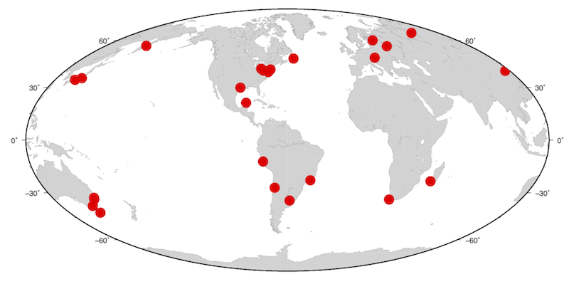
In addition to introducing early the fact that paleomagnetism contains a seriously scary number of acronyms, this exercise was meant to demonstrate that although the field is largely dipole, the non-dipolar components are significant over short time scales. Here’s a map of the localities selected by the students:
and here’s a map of where the VGPs for the modern day (2014) IGRF values for those localities plot compared to the modern geomagnetic pole.
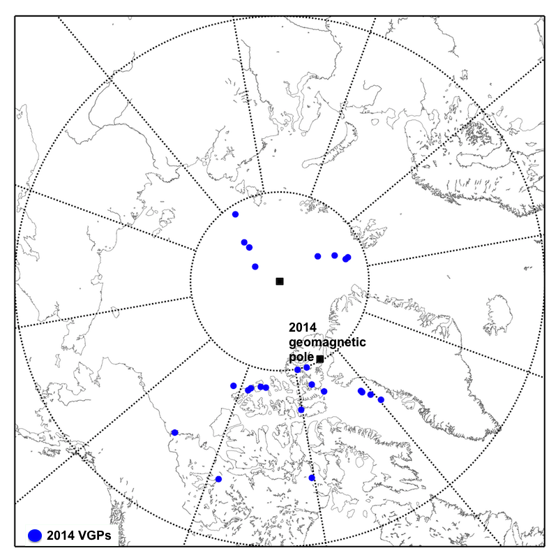
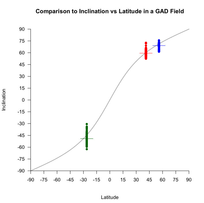
The point here is that the VGP calculation assumes a GAD field, whereas that is only the lowest order component of the spherical harmonic fit to the field encapsulated in the IGRF. At every locality, the quadrupole, octupole and even higher order components of the field contribute in varying amounts to the actual field direction and intensity, which skews them away from the geomagnetic pole (which is the estimated location of the IGRF dipole component). Another way to show this is to plot the IGRF-estimated inclinations from each locality against the simple tan(I)=2.tan(λ) relationship predicted for a GAD field.
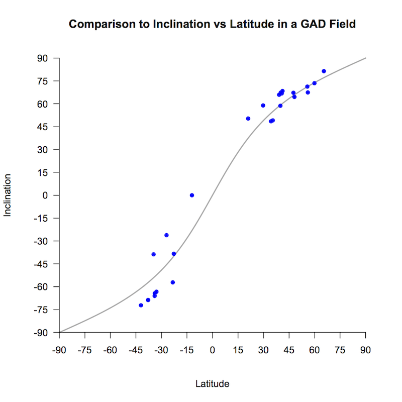
The fact that the data largely follow the predicted trend reflects the strong (~90%) contribution of the dipole component to the overall field; the scatter reflects the contribution of higher order components that make up the other 10%.
But what if we compare the present to the predicted values for 1914?
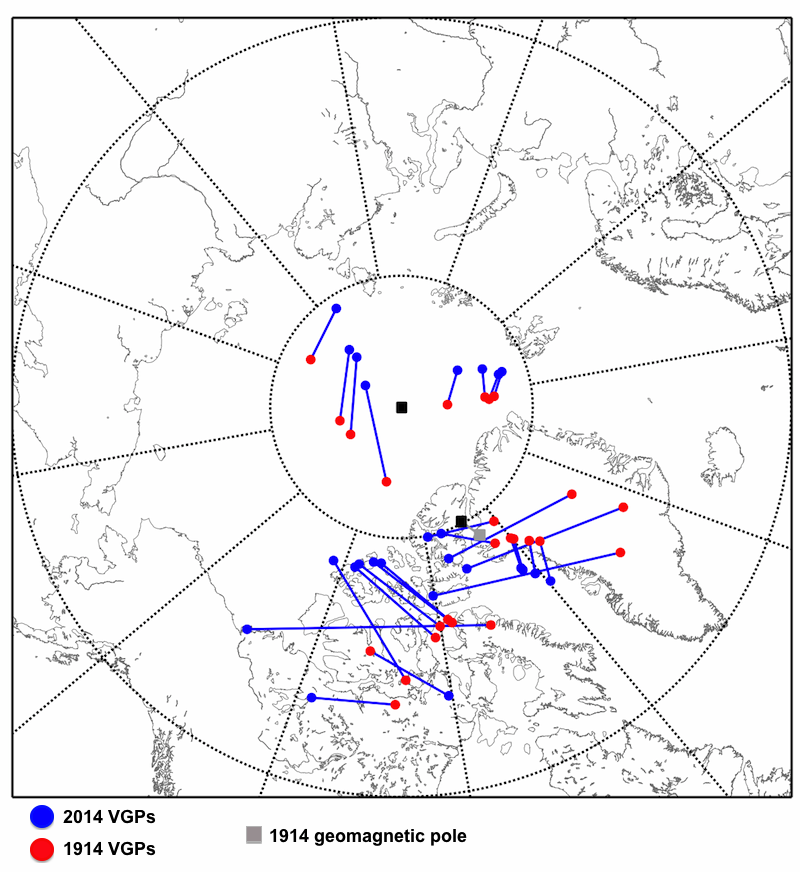
From this plot, we can see that the calculated VGPs for each locality move, but that not all of them move in the same direction, or at the same rate, and their motion is also different to the motion of the geomagnetic pole itself. Once again, we see the differing contribution of higher order field components at different locations of the Earth’s surface. But this plot also demonstrates that the field is time-varying, and that fluctuations in the higher order components are also generally larger over 100 year timescales than fluctuations in the dipole.
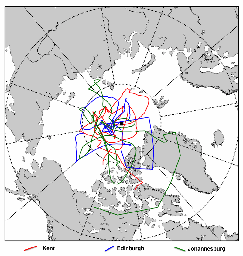
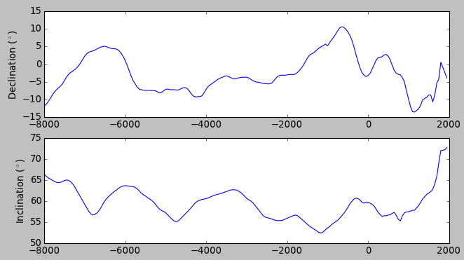
The final part of this exercise looked at secular variation (changes in the direction and magnitude of the magnetic field) over much longer timescales. I provided declination and inclination data from 8000 BCE to the present for three localities: Kent, Ohio; Edinburgh, UK; and Johannesburg, South Africa. This data was generated by the ‘igrf.py’ routine in Lisa Tauxe’s PMagPy suite, which uses the Holocene geomagnetic field model of Korte et al. (2011). Here, for example, are 10,000 years of predicted declination and inclination values for Kent:
The aim was to calculate VGPs for these data, then plot them up to see how they compared, like so:

What is apparent is that whereas the VGPs for each of the three locations have travelled their own individual path over the past 10,000 years, their aggregate behaviour is actually quite similar: namely, that the average position over 10,000 years of secular variation is centred on the geographic North poles – the Earth’s spin axis. Over a long enough time period, all the higher order variation of the field, which was clearly a big influence on the field you ‘see’ at any particular location on the Earth, seems to average out to zero, and we are left with a GAD field. Another way of looking at this to go back to the predicted inclination plot, which shows that for each of our three sites, the average inclination over 10,000 years is pretty consistent with a GAD field (although the average values still deviate a little, note).
Thus, so long as we are sampling over a long enough period, it appears that the GAD hypothesis is a reasonable one, making paleomagicians’ lives a little easier.