3.8 billion years! 4 billion years! 4.4 billion years! 4.57 billion years! When discussing the age of the Earth in introductory geology, I think it is important for students to know at least the basic principles of where these ages come from. That means explaining radiometric dating, which is consistently a challenging concept for students to get their heads around. This year, my attempts to come up with more useful ways to illustrate radioactive decay led me to code some simple visualisations in Python. I briefly describe them below, along with GIFs of the simulations themselves (they don’t loop but should replay if you open them or reload). Please feel free to use them if you find them useful; suggested improvements are also encouraged!
1: Radioactive decay as a random, and yet predictable, process
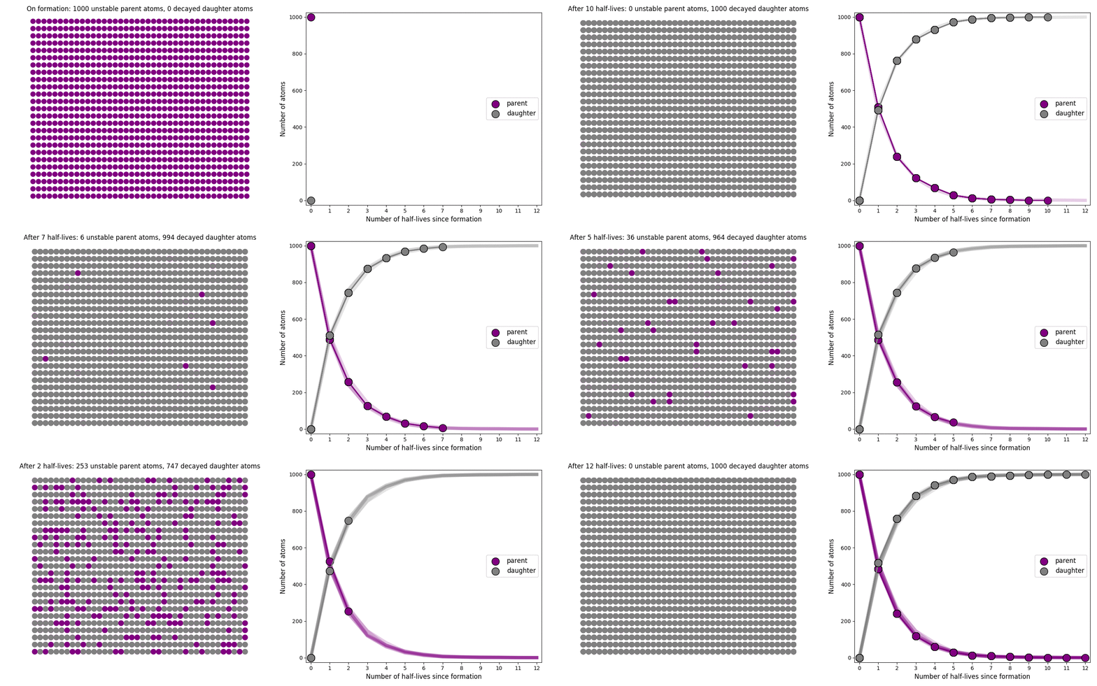
The basic simulation is a grid of 1000 purple parent atoms. Over each half life step, each parent has a 50-50 chance of decaying into a grey daughter atom. With 1000 atoms, you can nicely see how the proportions of parent to daughter change dramatically as the rock ages, and also see how the process completes after about ten half lives. Repeating the simulation multiple times helps to emphasise that:
– It is a random process: which atoms decay first, and which ones that survive the longest, changes between each simulation.
– The overall behaviour of this system is still predictable: the proportions of parent and daughter after each half life step stay roughly the same in each simulation. 1000 atoms is a bit on the small side for perfect statistical behaviour, but by adding the traces of previous runs you can see the average behaviour converges pretty well.

2: Different half-lives means very different rates of decay
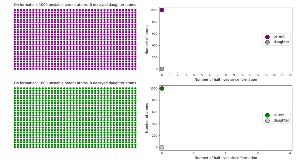
In this simulation, I’ve added a second grid of a green radioactive isotope, with a half life that is four times that of the purple atoms. This is an attempt to translate the more abstract ‘half-life’ concept into a physical length of time, and emphasise that different half lives mean different rates of change from parent to daughter. In this case, the purple atoms, which have the shorter half-life, quickly transform into their daughter atoms; the green atoms, with a considerably longer half-life transform much more slowly. This means that the green atoms persist (and can be used to date the rock by measuring their proportion relative to their daughter) long after the purple has all vanished (making it useless for dating).

(cross-posted to Highly Allochthonous)